library(tidytext)
library(tidyverse)

# Example text data
text_data <- data.frame(
  id = 1:3,
  text = c("Natural Language Processing is amazing!",
           "I love using R for text analysis.",
           "Text mining involves cleaning and processing text.")
)

# Tokenization
tokens <- text_data %>%
  unnest_tokens(word, text)

# Stop Word Removal
tokens <- tokens %>%
  anti_join(get_stopwords())

# Stemming
tokens <- tokens %>%
mutate(stem = SnowballC::wordStem(word))8 Natural Language Processing for Social Sciences
Natural Language Processing (NLP) is a subfield of artificial intelligence focused on the interaction between computers and human language (Jurafsky & Martin, 2008). In social sciences, NLP is used to analyze survey responses, study social media trends, and uncover insights from textual data.
8.1 Introduction to NLP
NLP enables the processing and analysis of large amounts of text data. By automating text analysis, researchers can extract patterns and insights that are difficult to discern manually.
8.2 Preprocessing Text Data
Text preprocessing is the foundation of NLP. It involves cleaning and preparing text for analysis.
8.2.1 Common Preprocessing Steps
8.3 Sentiment Analysis
Sentiment analysis identifies the emotional tone behind text data. The tidytext package makes it easy to conduct sentiment analysis.
# Use a sentiment lexicon
sentiments <- tokens %>%
  inner_join(get_sentiments("bing"))

# Summarize sentiment
sentiments %>%
  count(sentiment)
sentiment n
1 positive 28.4 Topic Modeling
Topic modeling uncovers latent themes in text data. Latent Dirichlet Allocation (LDA) is a popular algorithm for this purpose.
library(Matrix)
library(topicmodels)

# Create the `n` column
tokens_with_counts <- tokens %>%
  count(id, word)

# Generate DTM
dtm <- cast_dtm(tokens_with_counts, document = id, term = word, value = n)

# Apply Latent Dirichlet Allocation (LDA)
lda_model <- LDA(dtm, k = 2, control = list(seed = 123))  # `k` is the number of topics

# Extract topics
topics <- tidy(lda_model, matrix = "beta")  # "beta" represents word-topic probabilities
topics
# A tibble: 24 × 3
topic term beta
<int> <chr> <dbl>
1 1 amazing 0.0708
2 2 amazing 0.0625
3 1 language 0.0129
4 2 language 0.121
5 1 natural 0.0208
6 2 natural 0.113
7 1 processing 0.113
8 2 processing 0.153
9 1 analysis 0.0796
10 2 analysis 0.0537
# ℹ 14 more rows8.5 Word Embeddings
Word embeddings represent words as numerical vectors, capturing their meaning and relationships.
library(text2vec)

# Example tokenized data grouped by documents
documents <- split(tokens$word, tokens$id)

# Step 1: Create an iterator over tokenized documents
iter <- itoken(documents, progressbar = FALSE)

# Step 2: Create a vocabulary
vocab <- create_vocabulary(iter)

# Step 3: Prune vocabulary (optional, e.g., remove low-frequency words)
vocab <- prune_vocabulary(vocab, term_count_min = 2)

# Step 4: Create a vocabulary vectorizer
vectorizer <- vocab_vectorizer(vocab)

# Step 5: Create a Term-Cooccurrence Matrix (TCM)
tcm <- create_tcm(iter, vectorizer, skip_grams_window = 5)

# Step 6: Fit the GloVe model
glove <- GlobalVectors$new(rank = 50, x_max = 10)
word_vectors <- glove$fit_transform(tcm)
INFO [11:11:21.721] epoch 1, loss 0.4038
INFO [11:11:21.746] epoch 2, loss 0.2536
INFO [11:11:21.752] epoch 3, loss 0.1664
INFO [11:11:21.753] epoch 4, loss 0.1107
INFO [11:11:21.754] epoch 5, loss 0.0748
INFO [11:11:21.754] epoch 6, loss 0.0509
INFO [11:11:21.755] epoch 7, loss 0.0347
INFO [11:11:21.756] epoch 8, loss 0.0237
INFO [11:11:21.756] epoch 9, loss 0.0162
INFO [11:11:21.757] epoch 10, loss 0.0111# Combine main and context embeddings (optional)
word_vectors <- word_vectors + t(glove$components)
# View the word vectors
word_vectors["text", ] [1] -0.4865584679 0.5059907389 0.1219085168 -0.3972363103 0.2988029896
[6] -0.5209045688 -0.4974476420 0.2123235257 -0.3349718940 -0.0002986411
[11] -0.1540584652 -0.0814074061 0.5636523258 -0.1574191368 0.0149780471
[16] -0.2750642877 0.0372914495 -0.1495178341 0.6907387913 -0.1857780801
[21] 0.5673706071 0.2972066846 -0.0612599393 0.1283139135 -0.2839922940
[26] 0.3009238544 0.1481102999 0.6205589714 0.5189595583 0.0609683263
[31] 0.4187442669 0.1422638213 0.6580475972 -0.2777014929 0.5761448557
[36] -0.6724397621 -0.1266772683 0.1886747241 0.4412097288 -0.4117930484
[41] -0.5903334707 0.6189598248 -0.4125707645 -0.0069357213 -0.0361341009
[46] 0.7210115419 0.4413343812 0.0453418015 -0.0520747671 0.24749906878.6 Ethical Considerations in NLP
- Bias in Text Data: Models can inherit biases from training data, leading to skewed or unfair results.
- Privacy Concerns: Text analysis often involves sensitive or personal data, requiring ethical handling and anonymization.
8.7 Summary
In this chapter, we:
- Introduced NLP and its applications in social sciences.
- Explored key preprocessing steps like tokenization and stop word removal.
- Conducted sentiment analysis and topic modeling.
- Generated word embeddings for deeper text analysis.
8.8 Case Study: Sentiment Analysis of Social Media Posts
8.8.1 Introduction
Social media platforms are a valuable source of public opinion data. Analyzing the sentiment of posts can reveal how the public perceives events, policies, or brands. In this case study, we demonstrate how to preprocess text data and perform sentiment analysis using the tidytext package.
8.8.2 Objective
This case study demonstrates: 1. Preprocessing text data for analysis. 2. Conducting sentiment analysis with tidytext. 3. Visualizing sentiment distributions.
8.8.3 Dataset
We simulate a dataset of social media posts for this analysis.
# Simulated social media dataset
set.seed(123)
social_media <- data.frame(
  username = paste0("user", 1:100),
  date = sample(seq.Date(from = as.Date("2025-01-01"), to = as.Date("2025-01-10"), by = "day"), 100, replace = TRUE),
  text = sample(
    c(
      "I love this policy, it's so beneficial!",
      "This decision is terrible and harmful.",
      "I'm not sure how to feel about this change.",
      "Amazing initiative by the government!",
      "This policy is confusing and lacks clarity."
    ),
    100,
    replace = TRUE
  )
)

# View dataset
head(social_media)
username date text
1 user1 2025-01-03 I'm not sure how to feel about this change.
2 user2 2025-01-03 This decision is terrible and harmful.
3 user3 2025-01-10 This policy is confusing and lacks clarity.
4 user4 2025-01-02 This policy is confusing and lacks clarity.
5 user5 2025-01-06 I'm not sure how to feel about this change.
6 user6 2025-01-05 Amazing initiative by the government!8.8.4 Step 1: Preprocessing
library(tidytext)
library(dplyr)

# Tokenize text
tokens <- social_media %>%
  unnest_tokens(word, text)

# Remove stop words
tokens <- tokens %>%
  anti_join(get_stopwords(), by = "word")

# View processed tokens
head(tokens)
username date word
1 user1 2025-01-03 sure
2 user1 2025-01-03 feel
3 user1 2025-01-03 change
4 user2 2025-01-03 decision
5 user2 2025-01-03 terrible
6 user2 2025-01-03 harmful8.8.5 Step 2: Perform Sentiment Analysis
# Perform sentiment analysis
sentiments <- tokens %>%
  inner_join(get_sentiments("bing"), by = "word")

# Summarize sentiment
sentiment_summary <- sentiments %>%
  count(sentiment) %>%
  mutate(percentage = n / sum(n) * 100)

# View sentiment summary
sentiment_summary
sentiment n percentage
1 negative 90 50.84746
2 positive 87 49.152548.8.6 Step 3: Visualize Sentiment
library(ggplot2)

# Plot sentiment distribution
ggplot(sentiment_summary, aes(x = sentiment, y = percentage, fill = sentiment)) +
  geom_bar(stat = "identity", show.legend = FALSE) +
  labs(title = "Sentiment Distribution", x = "Sentiment", y = "Percentage") +
  theme_minimal()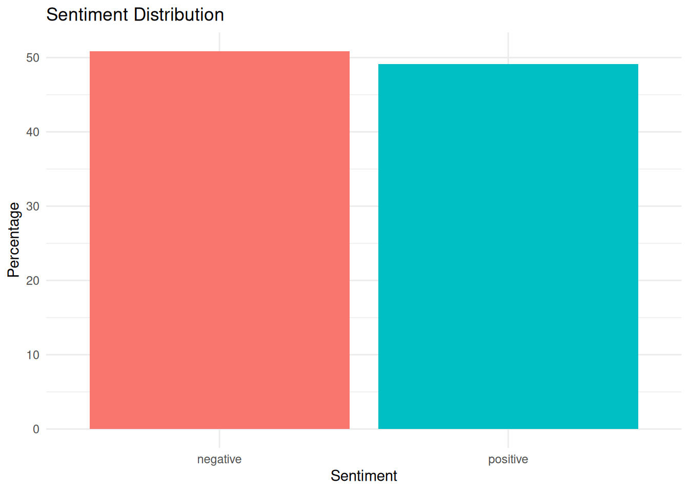
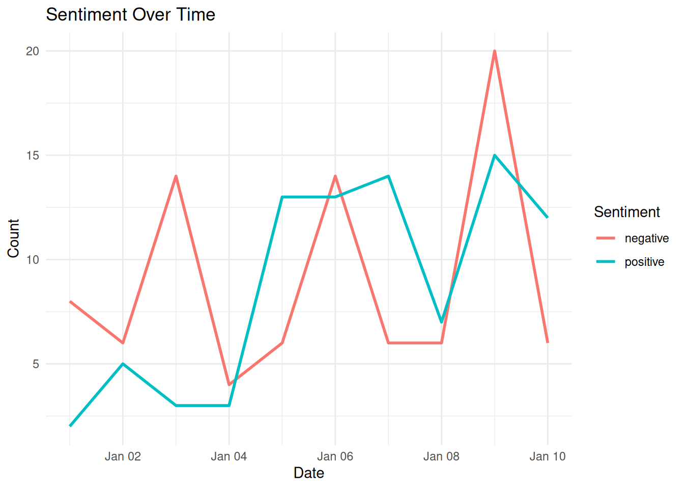
8.8.7 Step 4: Analyze Sentiment over Time
# Aggregate sentiment by date
sentiment_by_date <- sentiments %>%
  group_by(date, sentiment) %>%
  summarize(count = n(), .groups = "drop")

# Plot sentiment over time
ggplot(sentiment_by_date, aes(x = date, y = count, color = sentiment)) +
  geom_line(size = 1) +
  labs(title = "Sentiment Over Time", x = "Date", y = "Count", color = "Sentiment") +
  theme_minimal()