library(tidyverse)
library(haven)
df <- read_spss("data/james.sav")Research Review
Importing Data
Data was imported from spss file james.sav which was provided by Dr. Dellaneve:
Selecting Required Data
Some of the columns was omitted from dataset and a report from current variables and their frequency created as a PDF file and the data saved as a new data file:
#Removing Unnecessary Columns from Dataset (Tidying Dataset)
df <- df |>
  select(13:210) |>
  relocate(ID, 1) |>
  arrange(ID) |>
  relocate(q2z, q3z, q5z, .after = scale8)

#View the Cleaned Dataset:
sjPlot::view_df(df, show.frq = TRUE)

#Save Cleaned Data
saveRDS(df, "data/clean.rds")
Creating Categorical Variables
In this step, the categorical variables such as gender, race, education, etc. was created from related questions:
library(tidyverse)
library(sjlabelled)
library(sjPlot)

## Reading Clean Dataset:
df <- readRDS("data/clean.rds")

### Changing Management Status (Q136) to Categorical (manager)
df |>
  count(Q136)
df <- df |>
  mutate(manager = factor (case_when(
    Q136 == 1 ~ "manager",
    Q136 == 2 ~ "staff"
  ))) |>
    relocate(manager, .after = Q136)

### Changing Q2 to Gender (Factor = categorical)
df <- df |>
  mutate(gender = factor (case_when(Q2==1~"male",
                            Q2==2~"female",
                            Q2>2~NA))) |>
  relocate(gender, .after = Q2)

### Changing Q1 to Categorical Generation
df <- df |>
  mutate(generation = factor(case_when(Q1==1~"BabyBoomers",
                                Q1==2~"GenX",
                                Q1==3~"GenY",
                                Q1==4~"GenZ"
  ))) |>
  relocate(generation, .after = Q1)

## Changing Q3 to Categorical Race
df$race <- as_label(df$Q3, keep.labels = TRUE)
df <- df |>
  relocate(race, .after = Q3)

## Changing State to Categorical
df$states <- as_label(df$State, keep.labels = TRUE)
df <- df |>
  relocate(states, .after = State)

## Changing Q4 to Categorical Education
df$education <- as_label(df$Q4, keep.labels = TRUE)
df <- df |>
  relocate(education, .after = Q4)

## Change Q5 (Employment Status) to Categorical empstat
df$empstat <- as_label(df$Q5, keep.labels = TRUE)
df <- df |>
  relocate(empstat, .after = Q5)

## Changing Q6 to Categorical Industry
df$industry <- as_label(df$Q6, keep.labels = TRUE)
df <- df |>
  relocate(industry, .after = Q6)

## Save Transformed Clean Ready for Analysis Dataset
saveRDS(df, "data/transformd.rds")
Computing Continuous Variables
In this step, continuous (dependent) variables was calculated (took mean):
##Computing Variables of the Study as a New Pivot Table
library(tidyverse)
library(haven)
df <- readRDS("data/transformd.rds")
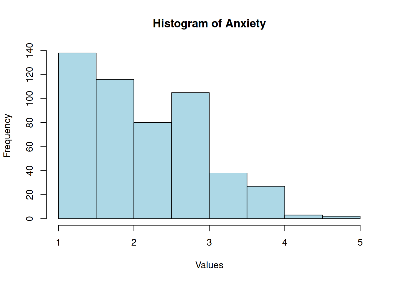
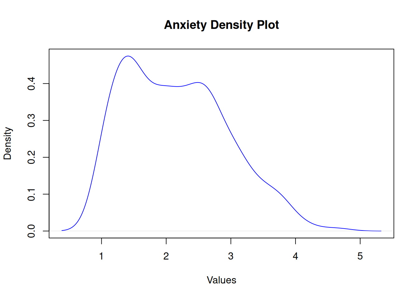
##Anxiety
df <- df |>
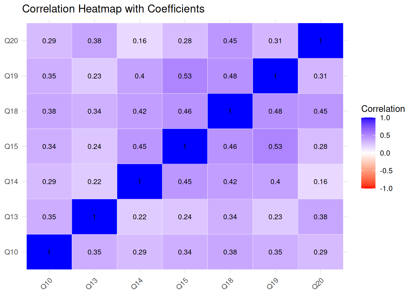
mutate(anxiety = round ((Q10 + Q13 + Q14 + Q15 + Q18 + Q19 + Q20)/7, 2),
.after = Q20)
##Avoidance
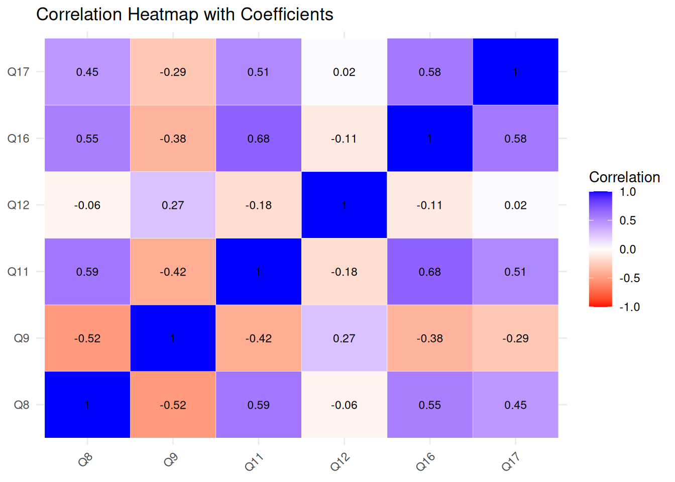
##1st Step: Reversing Questions 11, 8, 16, 17
df <- df |>
mutate(Q11New = 6 - Q11, .after = Q11) |>
mutate(Q8New = 6 - Q8, .after = Q8) |>
mutate(Q16New = 6 - Q16, .after = Q16) |>
mutate(Q17New = 6 - Q17, .after = Q17)
##2nd Step: Computing Avoidance from Revised Questions
df <- df |>
mutate(avoidance = round((Q9 + Q12 + Q8New + Q11New + Q16New + Q17New)/6, 2),
.after = Q17New)
##Interpersonal Deviance
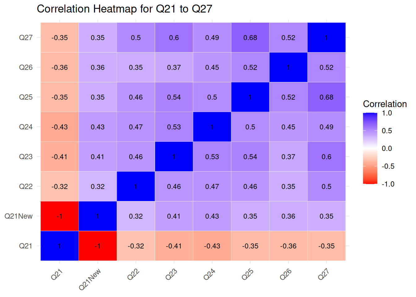
##1st Step: Revised Q21
df <- df |>
mutate(Q21New = 6 - Q21, .after = Q21)
##2nd Step: Interpersonal Deviance Variable
df <- df |>
mutate(intpersdev = round((rowSums(across(Q21New:Q27)))/7, 2), .after = Q27)
##Organizational Deviance
df <- df |>
mutate(orgdev = round((rowSums(across(Q28:Q39)))/12, 2), .after = Q39)
##ACE
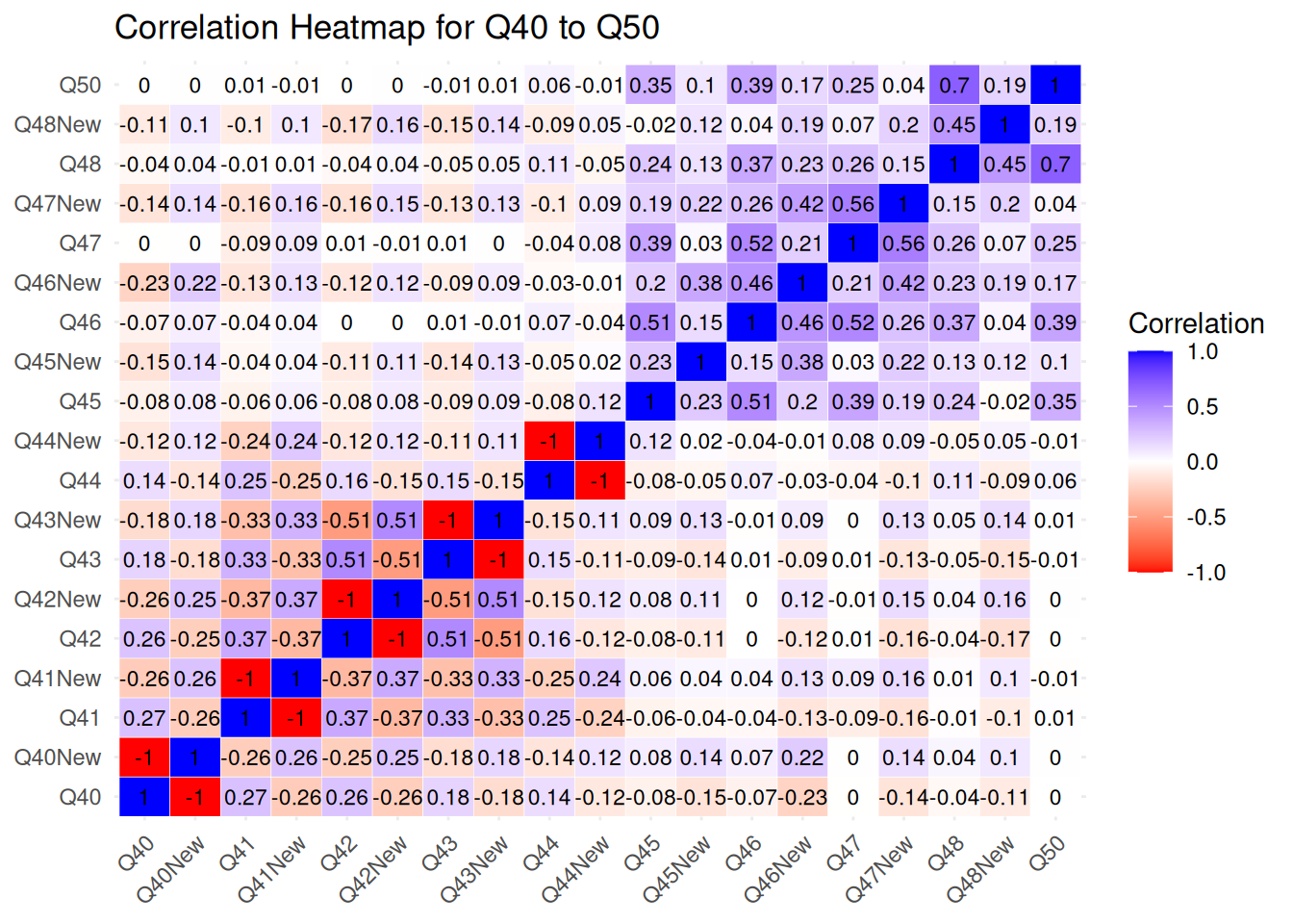
##1st Step: Reversing Q40-Q44 and Setting Missing Values(NA) for DK/DA values
df <- df |>
mutate(Q40New = case_when(Q40 == 1 ~ 2, Q40 == 2 ~1, Q40 == 3~0,
Q40 == 4~0), .after = Q40)
df <- df |>
mutate(Q41New = case_when(Q41 == 1 ~ 2, Q41 == 2 ~1, Q41 == 3~0,
Q41 == 4~0), .after = Q41)
df <- df |>
mutate(Q42New = case_when(Q42 == 1 ~ 2, Q42 == 2 ~1, Q42 == 3~0,
Q42 == 4~0), .after = Q42)
df <- df |>
mutate(Q43New = case_when(Q43 == 1 ~ 2, Q43 == 2 ~1, Q43 == 3~0,
Q43 == 4~0), .after = Q43)
df <- df |>
mutate(Q44New = case_when(Q44 == 1 ~ 2, Q44 == 2 ~1, Q44 == 3~0,
Q44 == 4~0), .after = Q44)
#2nd Step: Q45-Q50 Missing Values (NA) for DK/DA
df <- df |>
mutate(Q45New = case_when(Q45 == 1 ~ 1, Q45 == 2 ~2, Q45 == 3~3,
Q45 == 4~0, Q45 == 5~0), .after = Q45)
df <- df |>
mutate(Q46New = case_when(Q46 == 1 ~ 1, Q46 == 2 ~2, Q46 == 3~3,
Q46 == 4~0, Q46 == 5~0), .after = Q46)
df <- df |>
mutate(Q47New = case_when(Q47 == 1 ~ 1, Q47 == 2 ~2, Q47 == 3~3,
Q47 == 4~0, Q47 == 5~0), .after = Q47)
df <- df |>
mutate(Q48New = case_when(Q48 == 1 ~ 1, Q48 == 2 ~2, Q48 == 3~3,
Q48 == 4~0, Q48 == 5~0), .after = Q48)
df <- df |>
mutate(Q50New = case_when(Q50 == 1 ~ 1, Q50 == 2 ~2, Q50 == 3~3,
Q50 == 4~0, Q50 == 5~0), .after = Q50)
#3rd Step: Compute ACE from New Revised Questions
df <- df |>
mutate(ace = round((Q40New + Q41New + Q42New + Q43New + Q44New + Q45New
+Q46New + Q47New + Q48New + Q50New), 2), .after = Q50New)
##Phubbing
df <- df |>
mutate(phubbing = round((Q51 + Q52)/2, 2), .after = Q52)
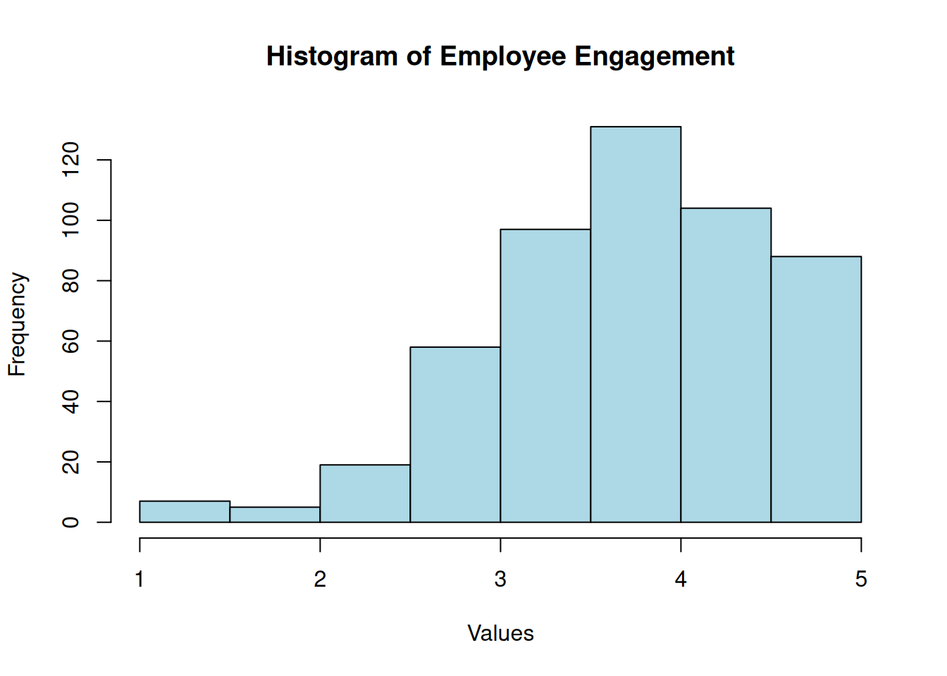
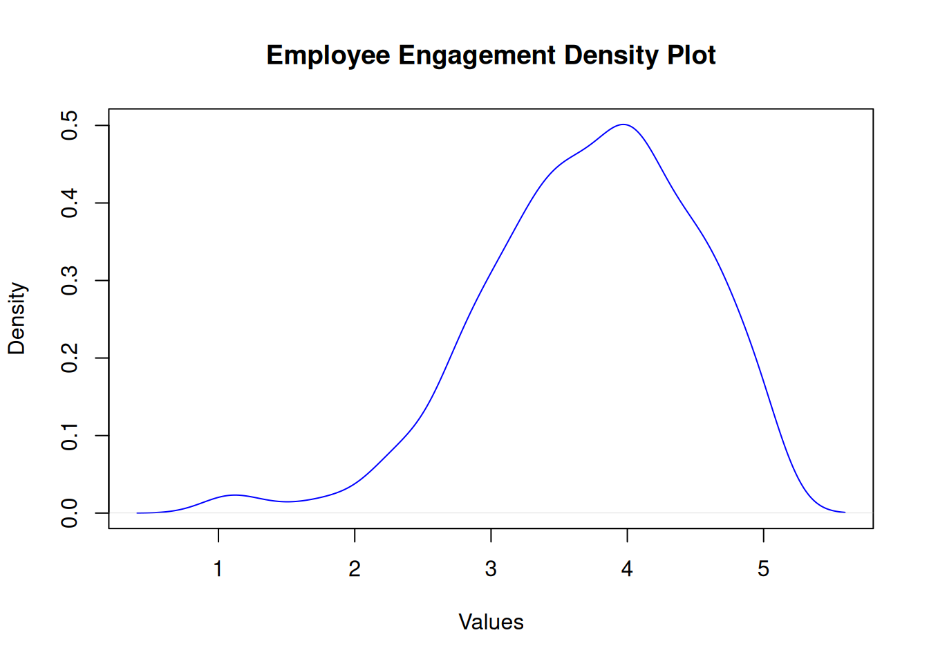
#Employee Engagement
df <- df |>
mutate(empengage = round((rowSums(across(Q60:Q100)))/41, 2), .after = Q100)
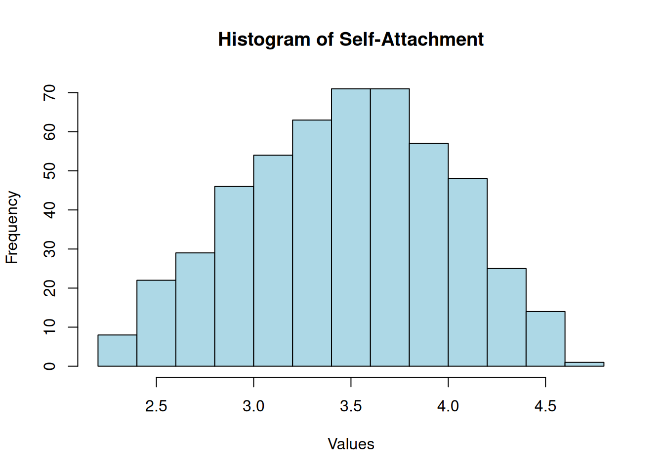
#Self-Attachment
##1st Step: Reversing Questions 102, 103, 104, 106, 107, 111
df <- df |>
mutate(Q102New = 6 - Q102, .after = Q102) |>
mutate(Q103New = 6 - Q103, .after = Q103) |>
mutate(Q104New = 6 - Q104, .after = Q104) |>
mutate(Q106New = 6 - Q106, .after = Q106) |>
mutate(Q107New = 6 - Q107, .after = Q107) |>
mutate(Q111New = 6 - Q111, .after = Q111)
##2nd Step: Computing Self-Attachment
df <- df |>
mutate(selfattach = (Q101 + Q102New + Q103New + Q104New + Q105 + Q106New +
Q107New + Q109 + Q111New + Q112)/10, .after = Q112)
#Remote
df <- df |>
mutate(remote = round((Q118 + Q119 + Q120)/3, 2), .after = Q120)
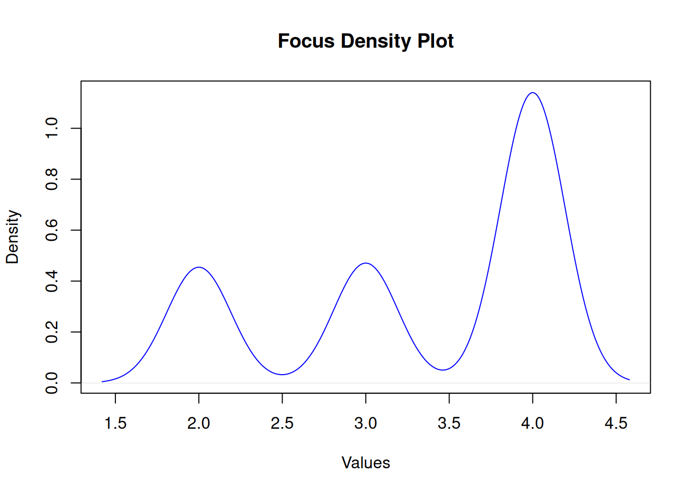
#Focus
df <- df |>
mutate(focus = (Q134 + Q135),
.after = Q135)
#Save File in CSV
write_csv(df, "data/variables.csv")Categorical Visualization
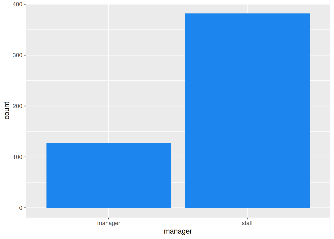
Management Status Bar Chart:
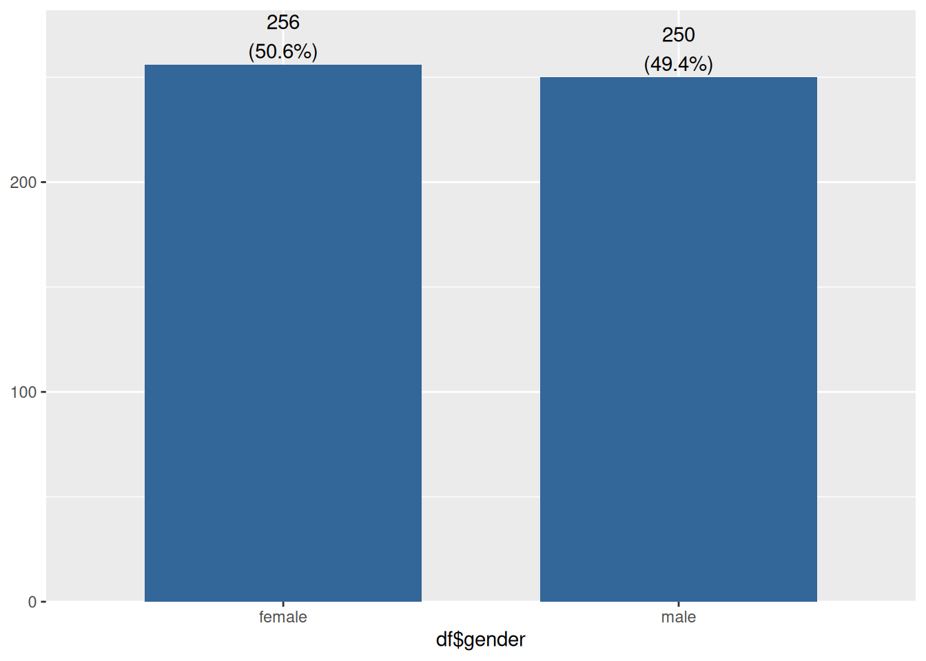
Gender Bar Charts:
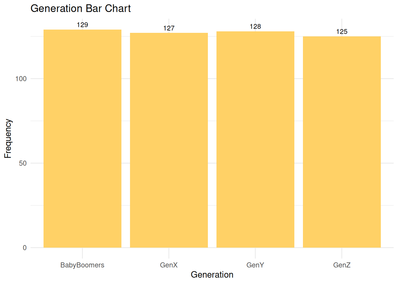
Generation
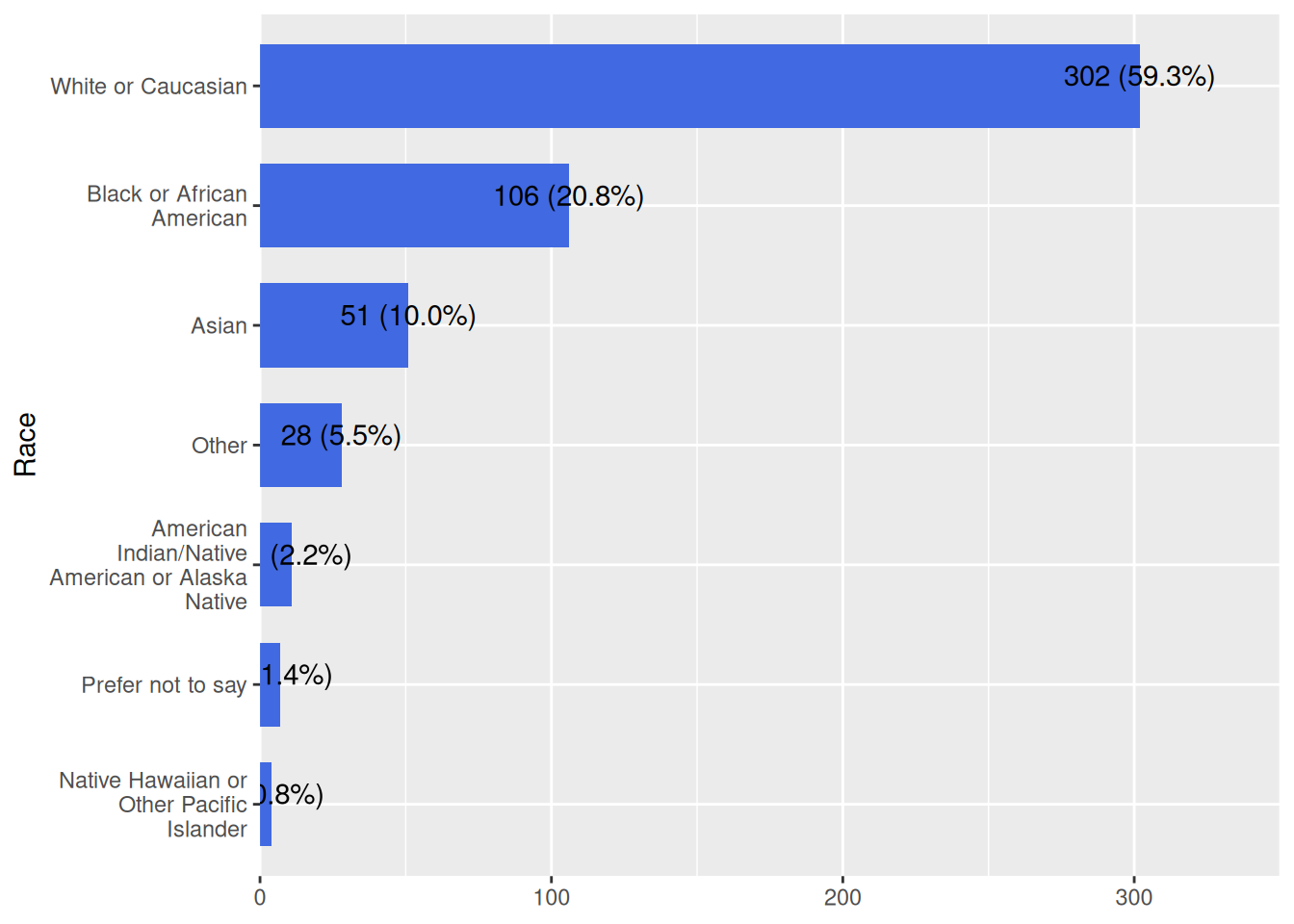
Race
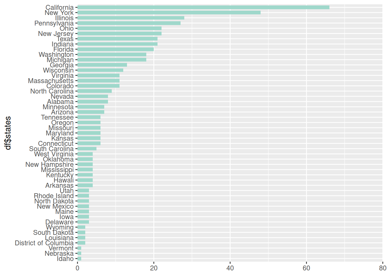
States
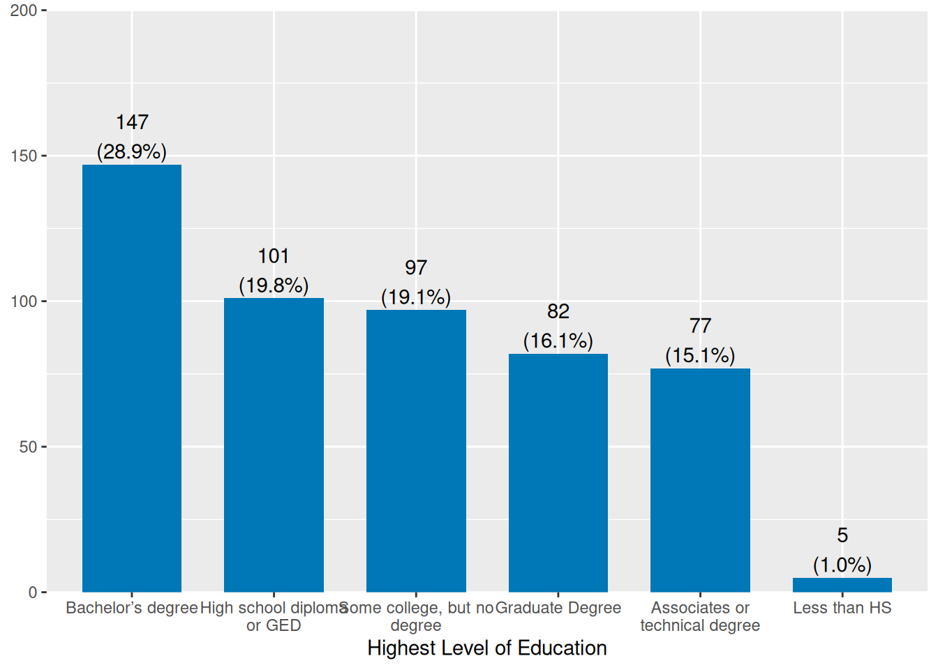
Education
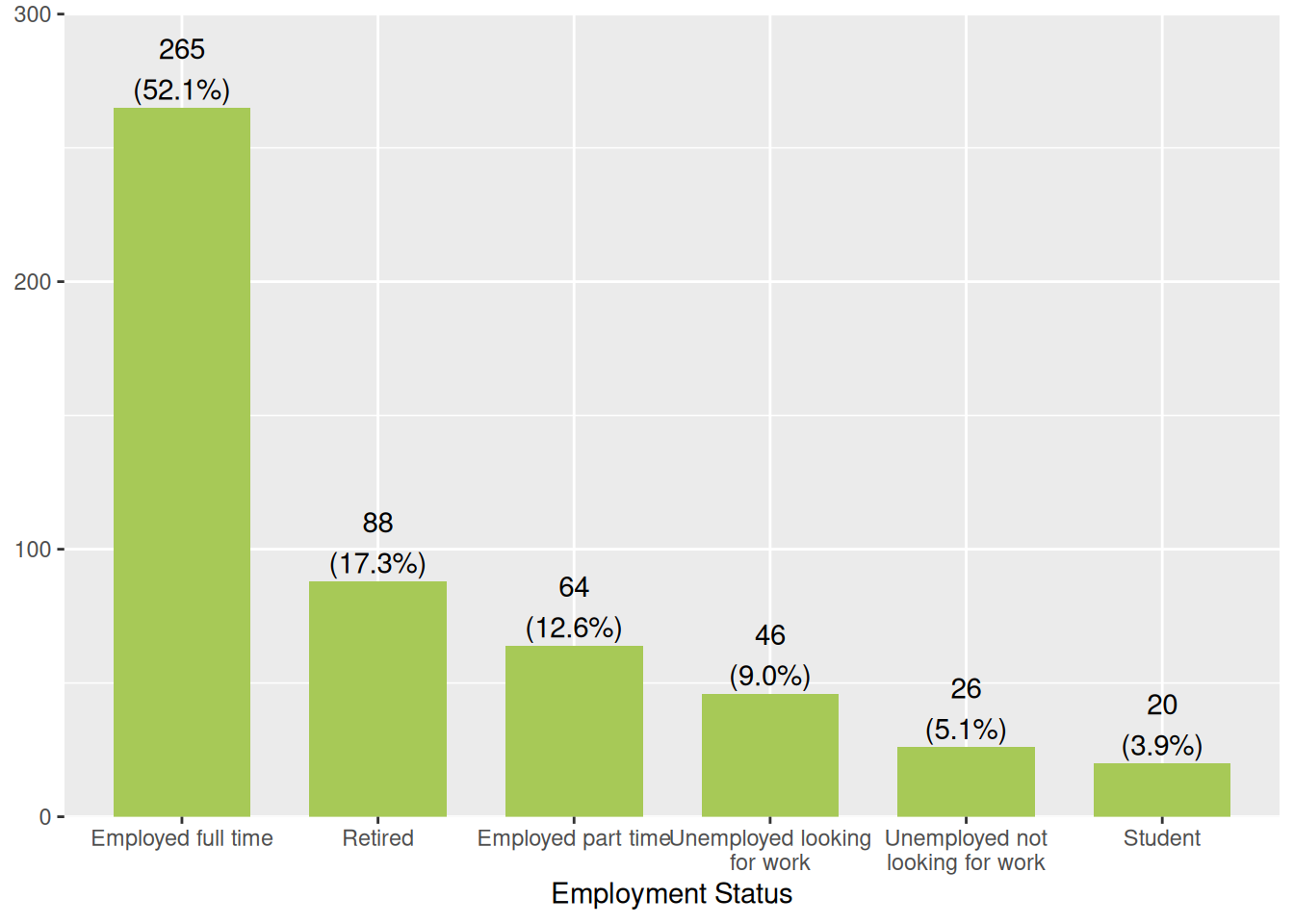
Employment Status
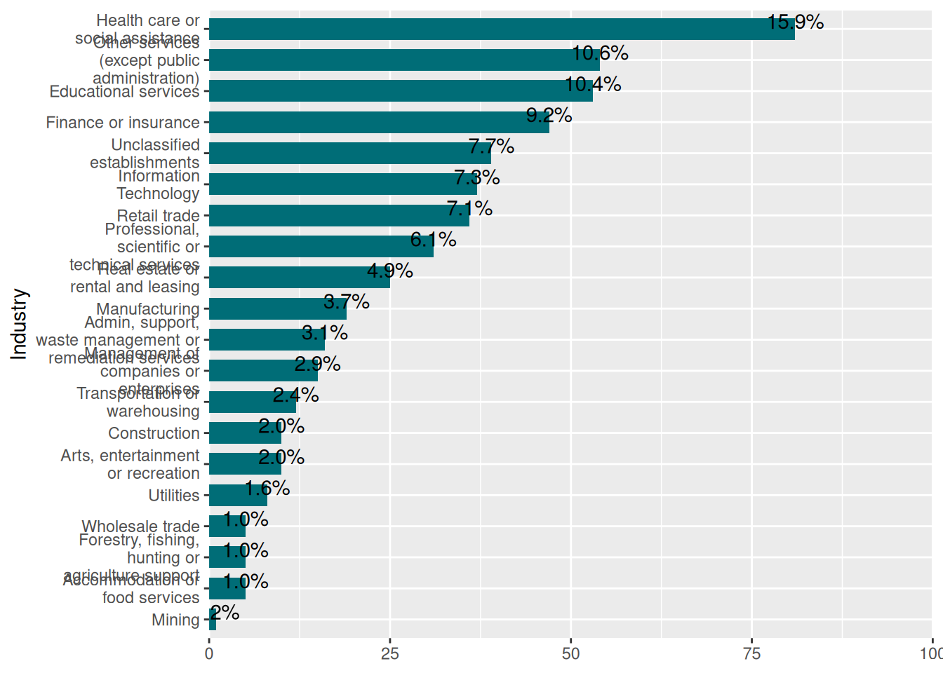
Industries
Spearman Correlations
In this step the Spearman correlations between questions of the study is created:
Anxiety Items
Avoidance Items
Interpersonal Deviance Items
ACE Items
Self-Attachment Items
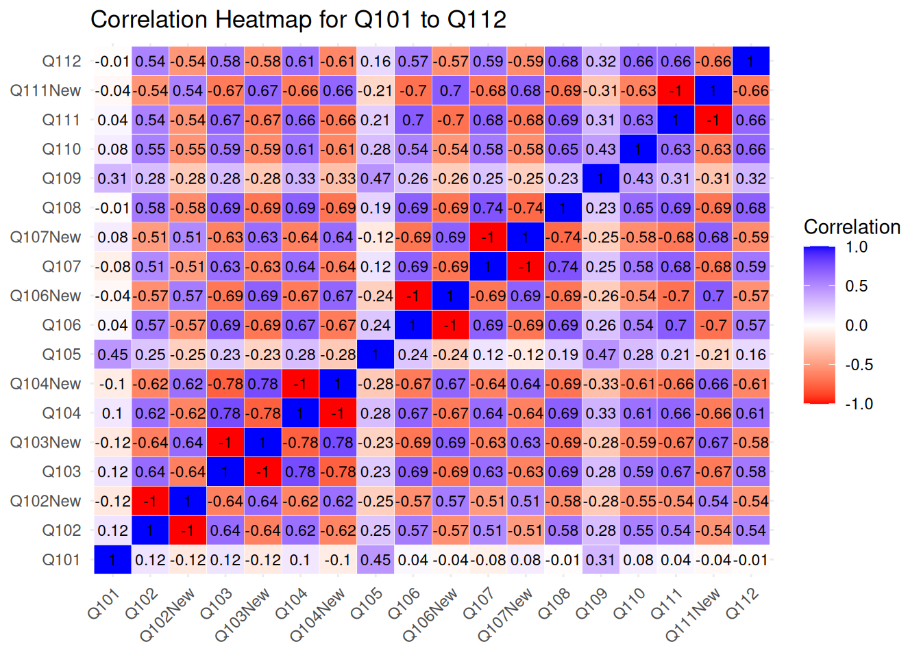
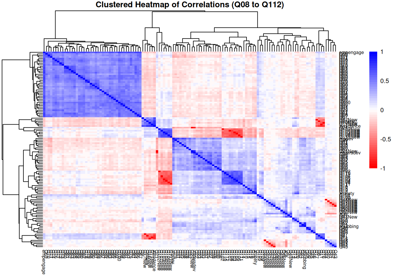
All Items (Q08 to Q112)
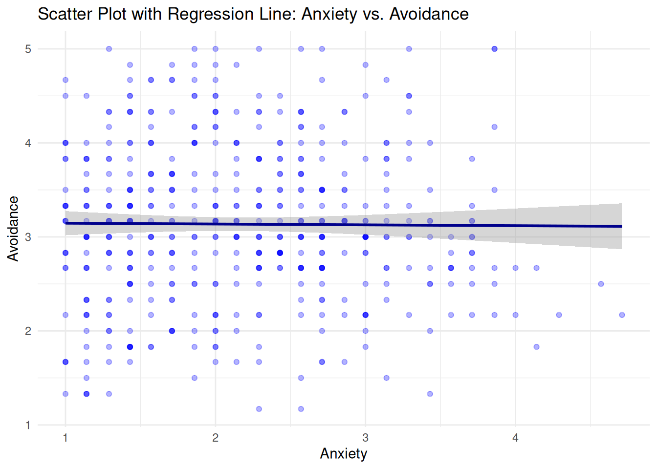
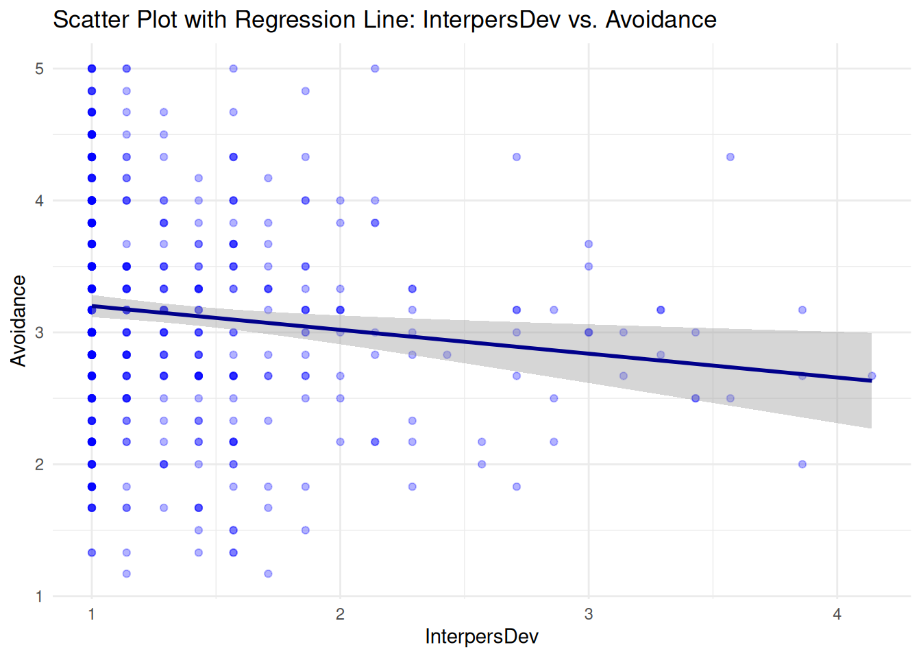
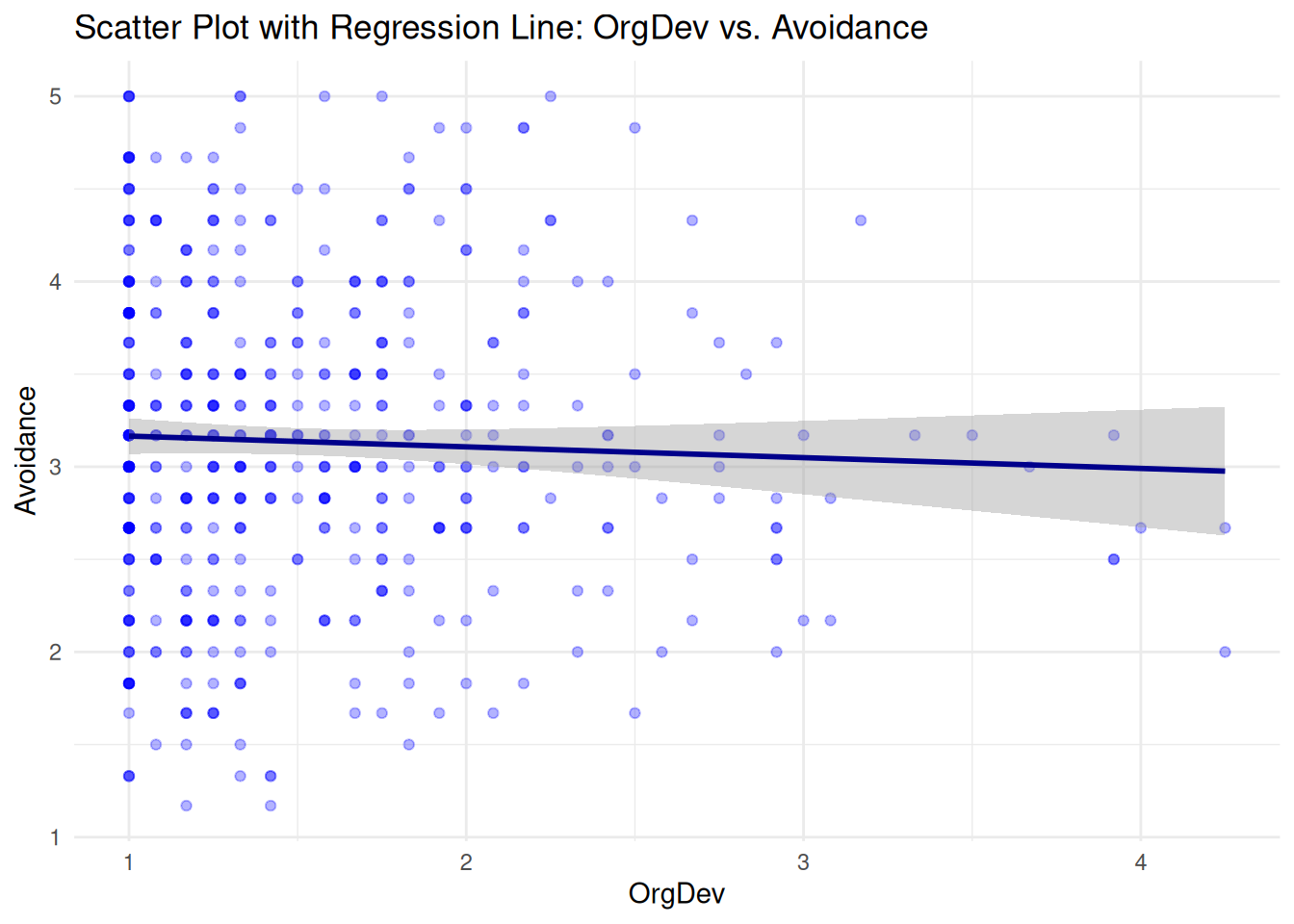
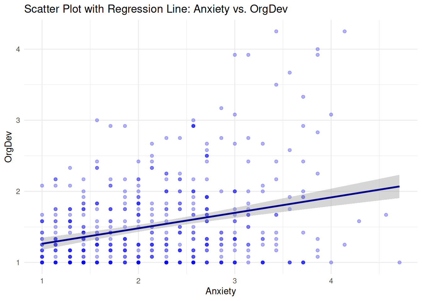
Scatter Plots
Anxiety vs. Avoidance
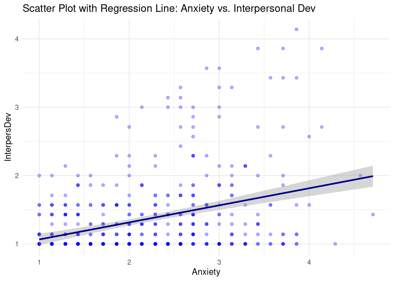
Interpersonal Deviance vs. Anxiety
Interpersonal Deviance vs. Avodiance
Organizational Deviance vs. Avoidance
OrgDev vs. Anxiety
Test of Normality
Employee Engagement
    Shapiro-Wilk normality test

data:  df$empengage
W = 1, p-value = 8e-09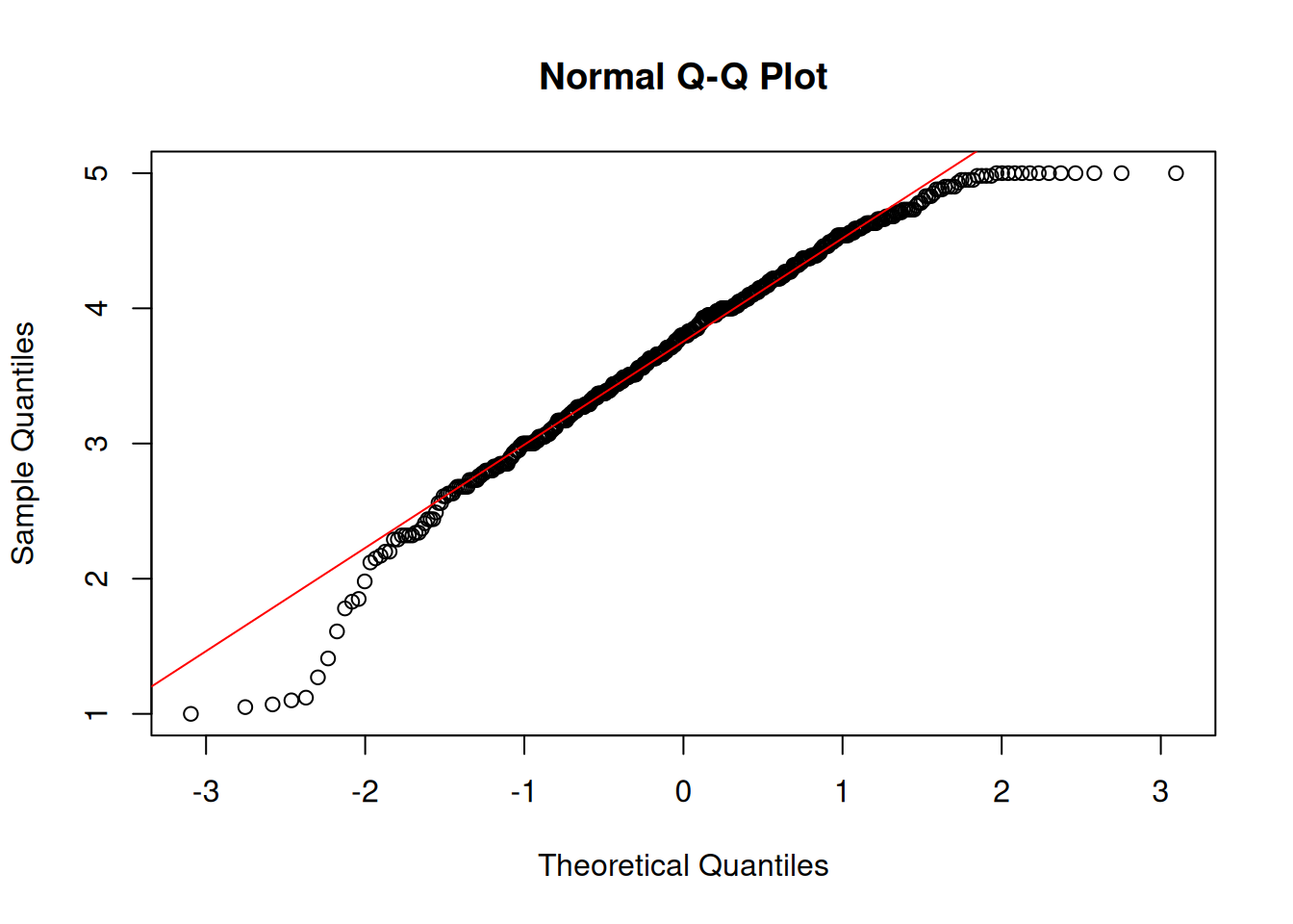
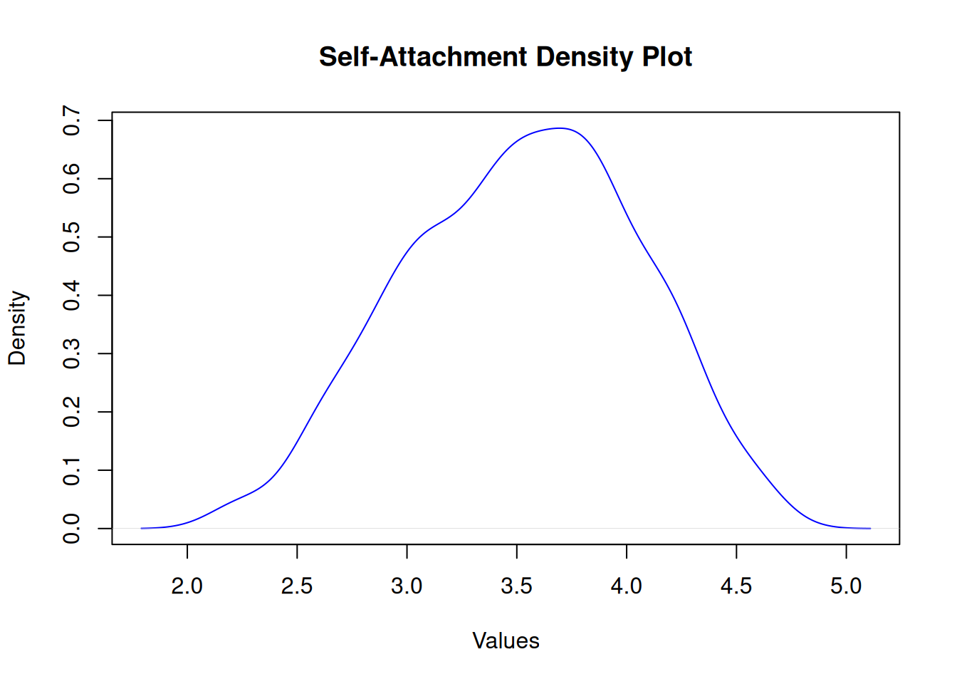
Self-Attachment
    Shapiro-Wilk normality test

data:  df$selfattach
W = 1, p-value = 2e-04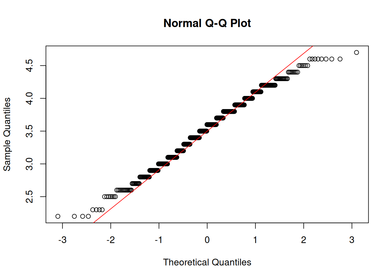
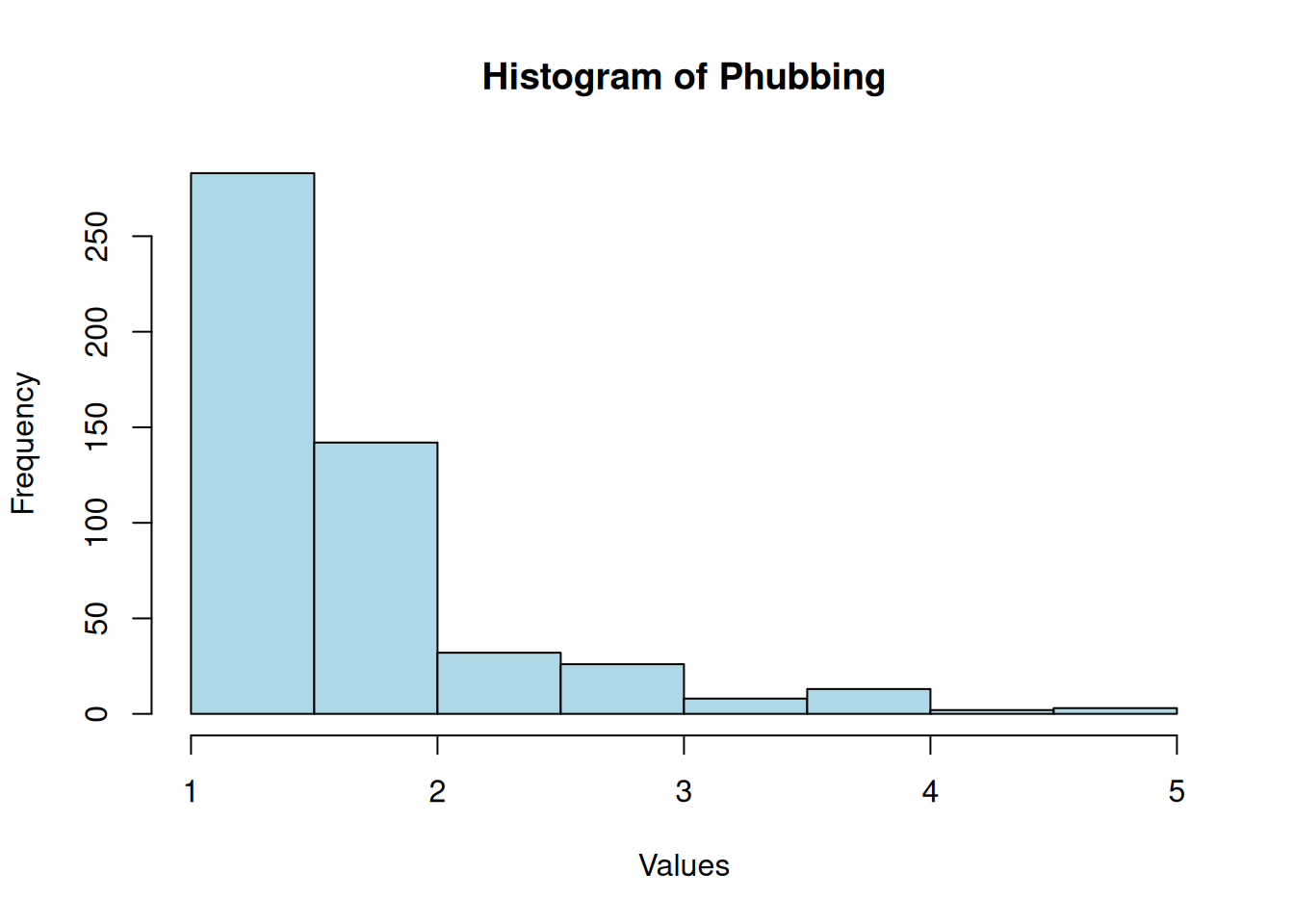
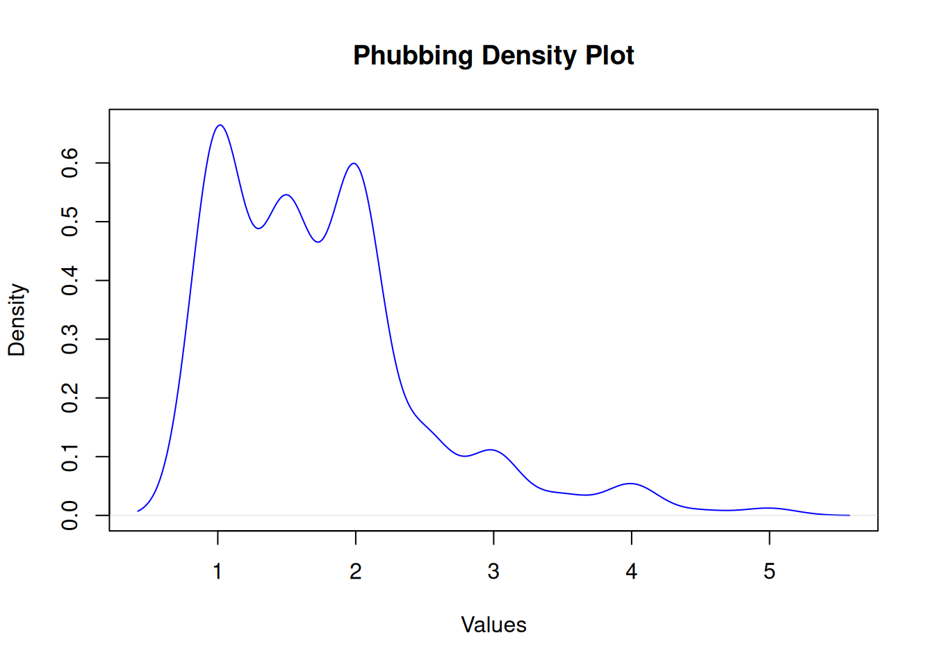
Phubbing
    Shapiro-Wilk normality test

data:  df$phubbing
W = 0.8, p-value <2e-16
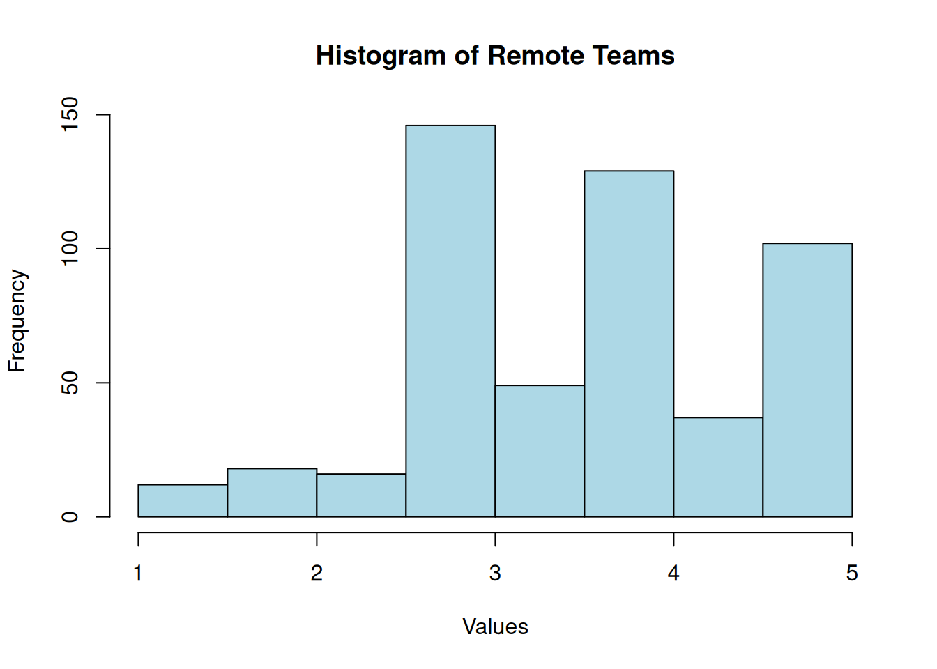
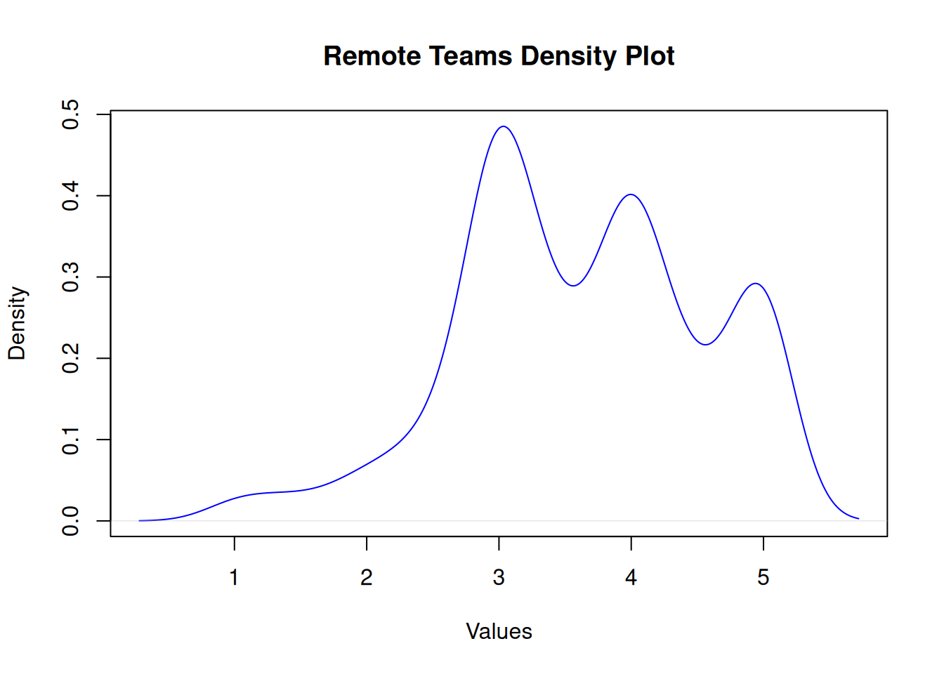
Remote Teams
    Shapiro-Wilk normality test

data:  df$remote
W = 0.9, p-value = 9e-13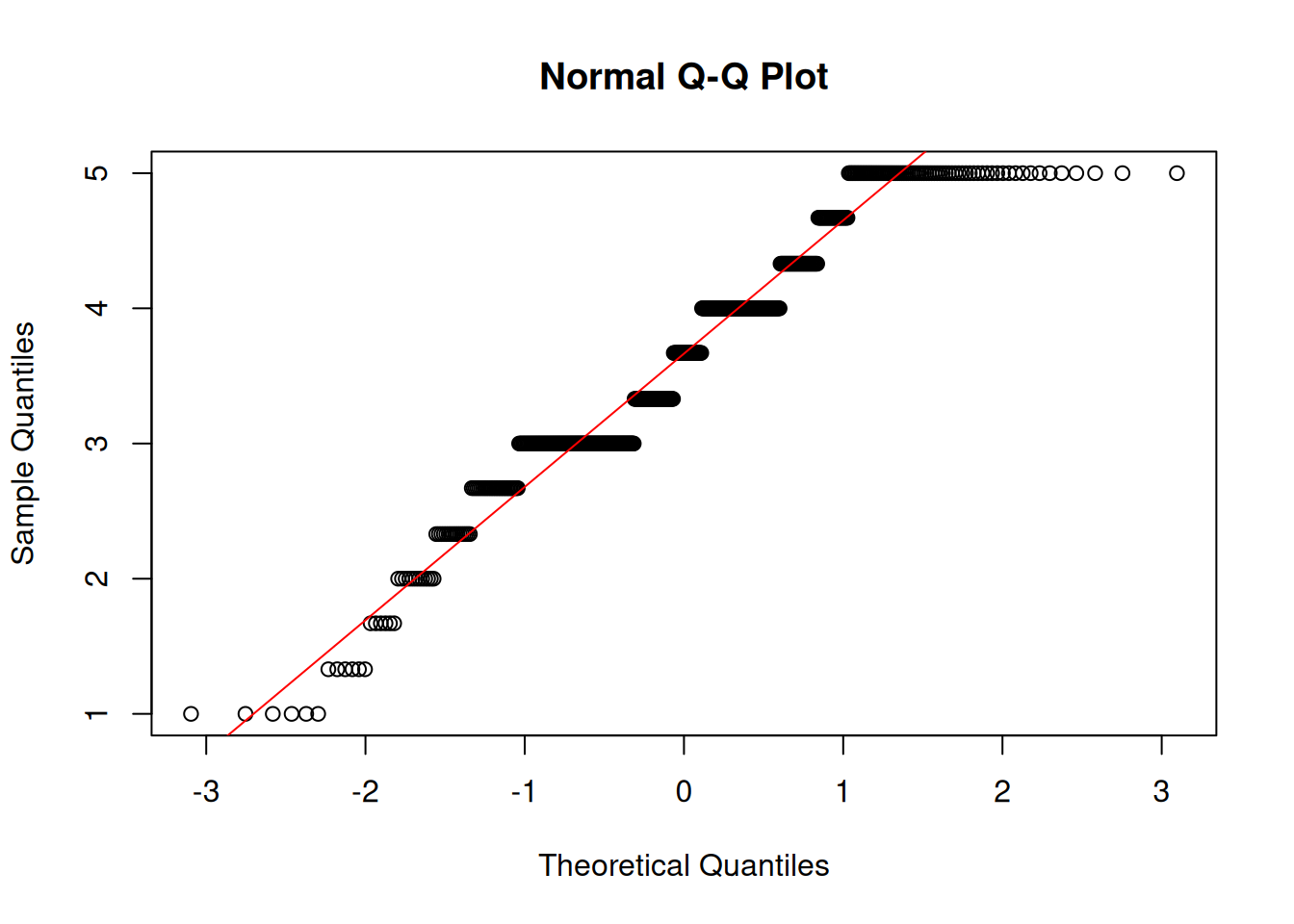
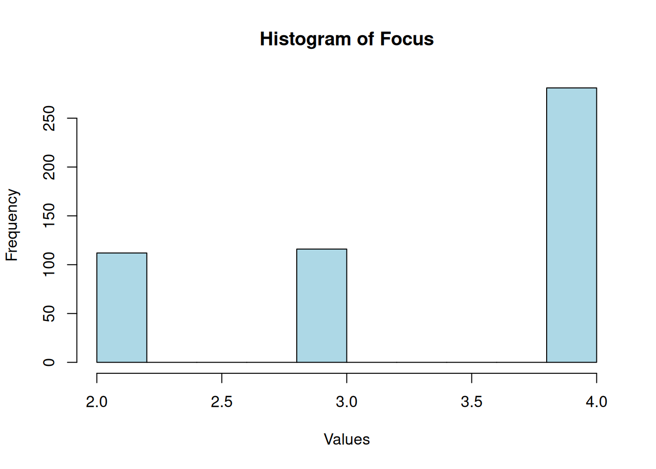
Focus
    Shapiro-Wilk normality test

data:  df$focus
W = 0.7, p-value <2e-16
Anxiety
    Shapiro-Wilk normality test

data:  df$anxiety
W = 1, p-value = 1e-10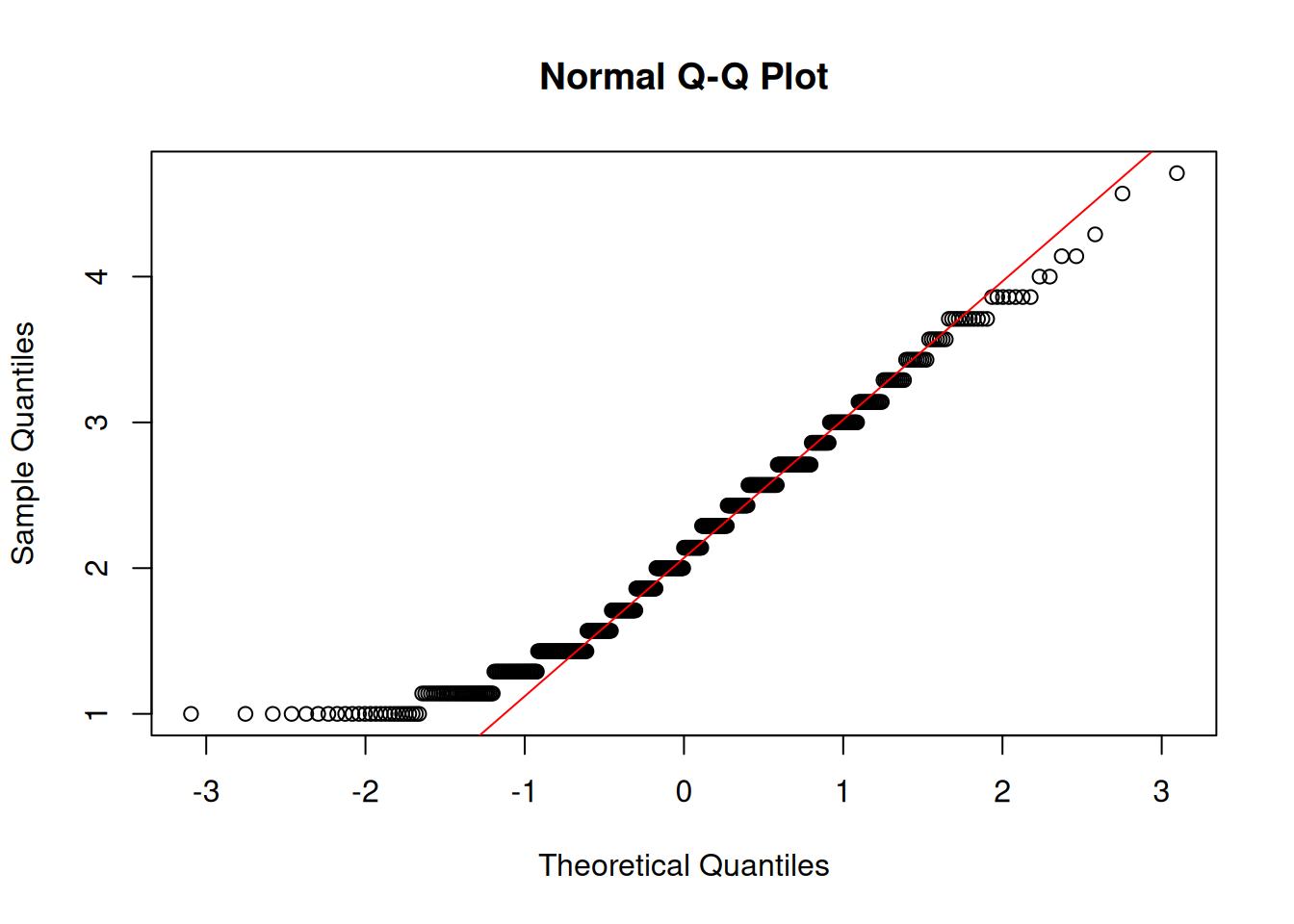
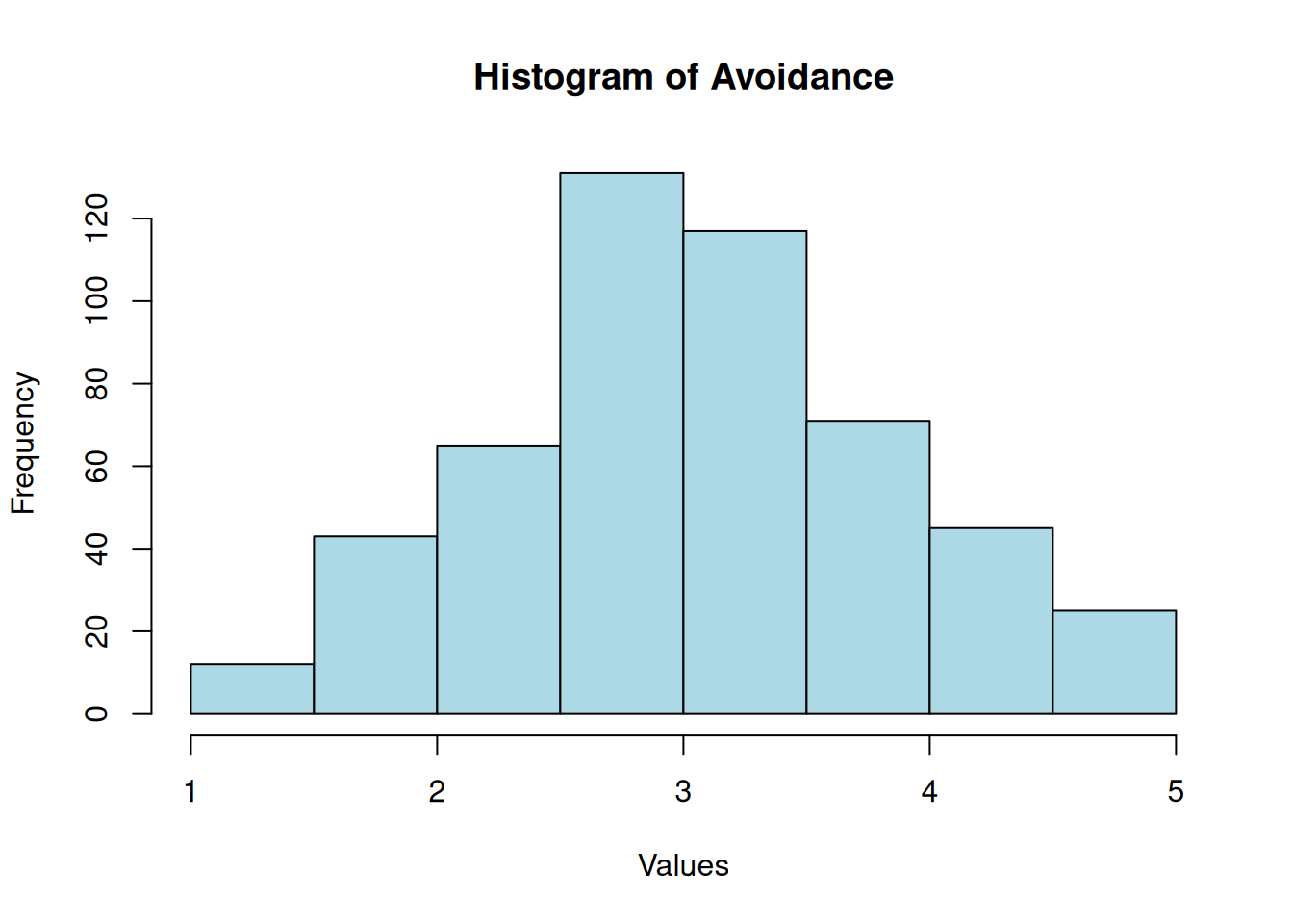
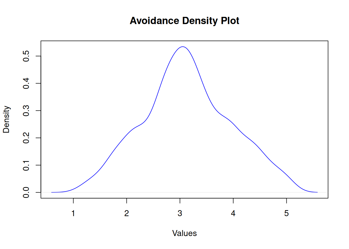
Avoidance
    Shapiro-Wilk normality test

data:  df$avoidance
W = 1, p-value = 3e-04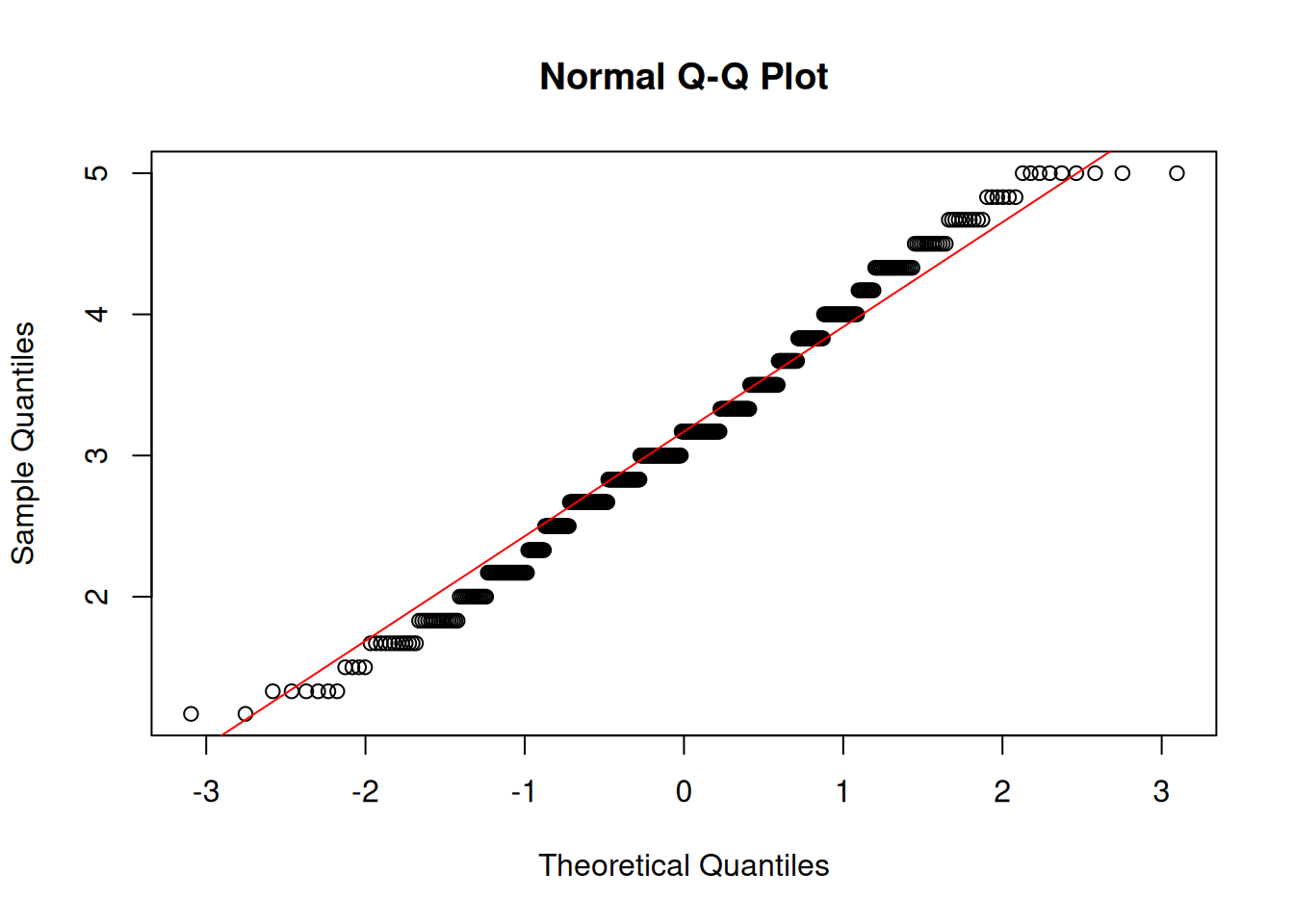
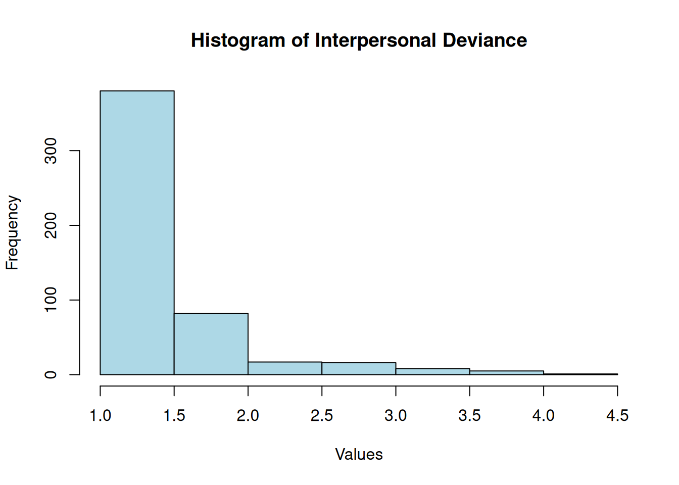
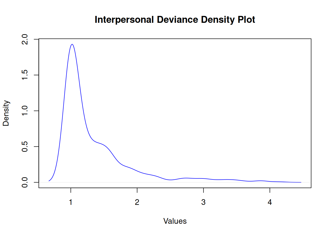
Interpersonal Deviance
    Shapiro-Wilk normality test

data:  df$intpersdev
W = 0.7, p-value <2e-16
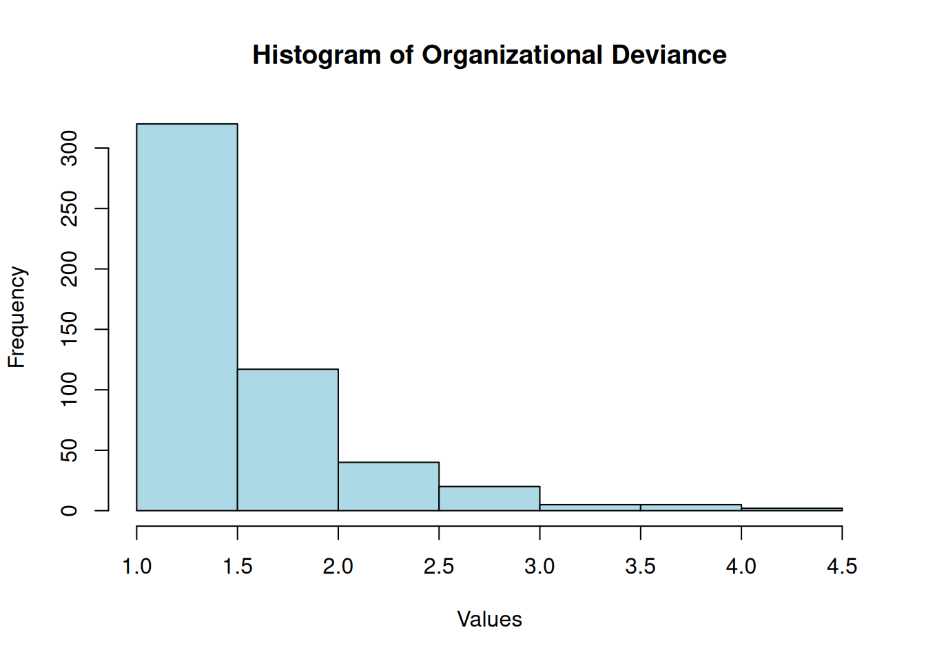
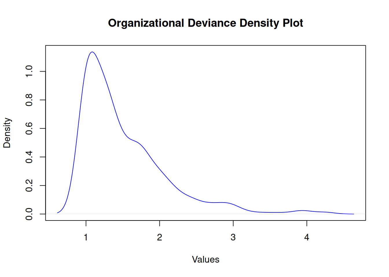
Organizational Deviance
    Shapiro-Wilk normality test

data:  df$orgdev
W = 0.8, p-value <2e-16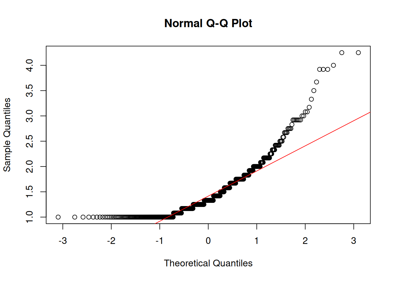
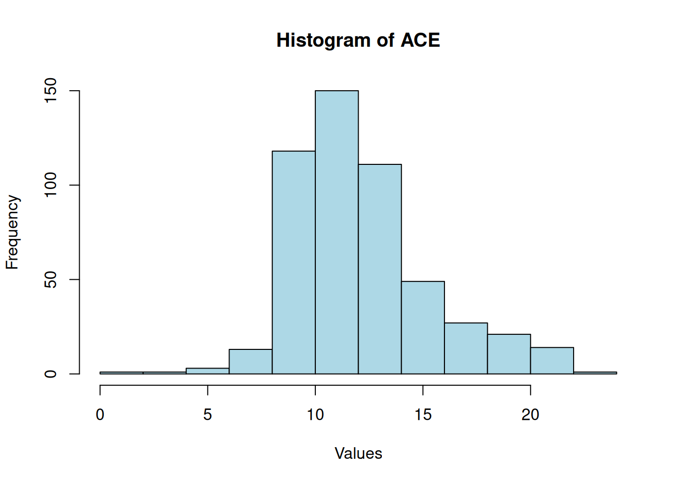
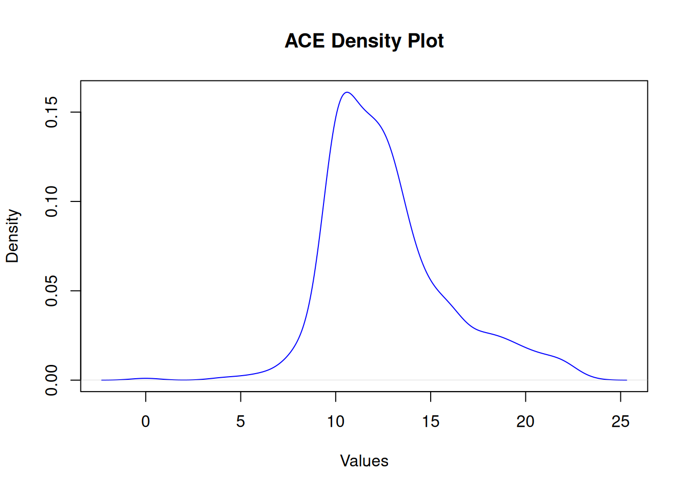
ACE
    Shapiro-Wilk normality test

data:  df$ace
W = 0.9, p-value = 1e-15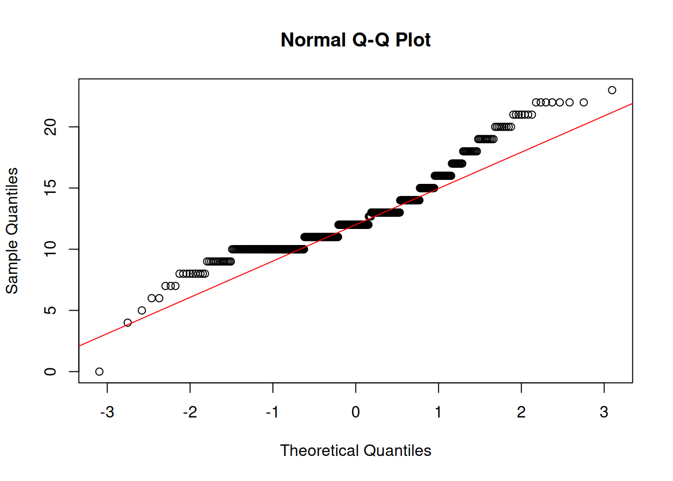
Kruskal Wallis Test
Since our continuous variables are not normally distributed, we used non-parametric test of Kruskal Wallis to find how the variables diverse among demographics:
Employee Engagement Vs. Demographics
As we see in the following results there is not any significant difference regarding employee engagement among demographics:
    Asymptotic Kruskal-Wallis Test

data:  empengage by
     race (American Indian/Native American or Alaska Native, Asian, Black or African American, Native Hawaiian or Other Pacific Islander, Other, Prefer not to say, White or Caucasian)
chi-squared = 10, df = 6, p-value = 0.1
    Asymptotic Kruskal-Wallis Test

data:  empengage by
     education (Associates or technical degree, Bachelor’s degree, Graduate Degree, High school diploma or GED, Some college, but no degree, Less than HS)
chi-squared = 5, df = 5, p-value = 0.5
    Asymptotic Kruskal-Wallis Test

data:  empengage by
     generation (BabyBoomers, GenX, GenY, GenZ)
chi-squared = 5, df = 3, p-value = 0.2
    Asymptotic Kruskal-Wallis Test

data:  empengage by gender (female, male)
chi-squared = 0.04, df = 1, p-value = 0.8
Self-Attachment Vs. Demographics
As the following results show, the self-attachment difference is significant for education and generation at p = 0.05
    Asymptotic Kruskal-Wallis Test

data:  selfattach by
     race (American Indian/Native American or Alaska Native, Asian, Black or African American, Native Hawaiian or Other Pacific Islander, Other, Prefer not to say, White or Caucasian)
chi-squared = 6, df = 6, p-value = 0.5
    Asymptotic Kruskal-Wallis Test

data:  selfattach by
     education (Associates or technical degree, Bachelor’s degree, Graduate Degree, High school diploma or GED, Some college, but no degree, Less than HS)
chi-squared = 19, df = 5, p-value = 0.002
    Asymptotic Kruskal-Wallis Test

data:  selfattach by
     generation (BabyBoomers, GenX, GenY, GenZ)
chi-squared = 55, df = 3, p-value = 6e-12
    Asymptotic Kruskal-Wallis Test

data:  selfattach by gender (female, male)
chi-squared = 4, df = 1, p-value = 0.05
Phubbing
The results below show that phubbing has a significant difference in generation.
    Asymptotic Kruskal-Wallis Test

data:  phubbing by
     race (American Indian/Native American or Alaska Native, Asian, Black or African American, Native Hawaiian or Other Pacific Islander, Other, Prefer not to say, White or Caucasian)
chi-squared = 3, df = 6, p-value = 0.8
    Asymptotic Kruskal-Wallis Test

data:  phubbing by
     education (Associates or technical degree, Bachelor’s degree, Graduate Degree, High school diploma or GED, Some college, but no degree, Less than HS)
chi-squared = 4, df = 5, p-value = 0.5
    Asymptotic Kruskal-Wallis Test

data:  phubbing by
     generation (BabyBoomers, GenX, GenY, GenZ)
chi-squared = 25, df = 3, p-value = 2e-05
    Asymptotic Kruskal-Wallis Test

data:  phubbing by gender (female, male)
chi-squared = 2, df = 1, p-value = 0.2
Remote Teams
Results indicate a significant difference for Remote Teams regarding generation
    Asymptotic Kruskal-Wallis Test

data:  remote by
     race (American Indian/Native American or Alaska Native, Asian, Black or African American, Native Hawaiian or Other Pacific Islander, Other, Prefer not to say, White or Caucasian)
chi-squared = 9, df = 6, p-value = 0.2
    Asymptotic Kruskal-Wallis Test

data:  remote by
     education (Associates or technical degree, Bachelor’s degree, Graduate Degree, High school diploma or GED, Some college, but no degree, Less than HS)
chi-squared = 6, df = 5, p-value = 0.3
    Asymptotic Kruskal-Wallis Test

data:  remote by
     generation (BabyBoomers, GenX, GenY, GenZ)
chi-squared = 12, df = 3, p-value = 0.009
    Asymptotic Kruskal-Wallis Test

data:  remote by gender (female, male)
chi-squared = 0.08, df = 1, p-value = 0.8
Focus
Results indicate focus has a significant difference regarding generation
    Asymptotic Kruskal-Wallis Test

data:  focus by
     race (American Indian/Native American or Alaska Native, Asian, Black or African American, Native Hawaiian or Other Pacific Islander, Other, Prefer not to say, White or Caucasian)
chi-squared = 10, df = 6, p-value = 0.1
    Asymptotic Kruskal-Wallis Test

data:  focus by
     education (Associates or technical degree, Bachelor’s degree, Graduate Degree, High school diploma or GED, Some college, but no degree, Less than HS)
chi-squared = 4, df = 5, p-value = 0.6
    Asymptotic Kruskal-Wallis Test

data:  focus by
     generation (BabyBoomers, GenX, GenY, GenZ)
chi-squared = 28, df = 3, p-value = 3e-06
    Asymptotic Kruskal-Wallis Test

data:  focus by gender (female, male)
chi-squared = 2, df = 1, p-value = 0.1
Anxiety
Anxiety shows a significant difference in generation and gender
    Asymptotic Kruskal-Wallis Test

data:  anxiety by
     race (American Indian/Native American or Alaska Native, Asian, Black or African American, Native Hawaiian or Other Pacific Islander, Other, Prefer not to say, White or Caucasian)
chi-squared = 5, df = 6, p-value = 0.5
    Asymptotic Kruskal-Wallis Test

data:  anxiety by
     education (Associates or technical degree, Bachelor’s degree, Graduate Degree, High school diploma or GED, Some college, but no degree, Less than HS)
chi-squared = 6, df = 5, p-value = 0.3
    Asymptotic Kruskal-Wallis Test

data:  anxiety by
     generation (BabyBoomers, GenX, GenY, GenZ)
chi-squared = 39, df = 3, p-value = 2e-08
    Asymptotic Kruskal-Wallis Test

data:  anxiety by gender (female, male)
chi-squared = 5, df = 1, p-value = 0.03
Avoidance
    Asymptotic Kruskal-Wallis Test

data:  avoidance by
     race (American Indian/Native American or Alaska Native, Asian, Black or African American, Native Hawaiian or Other Pacific Islander, Other, Prefer not to say, White or Caucasian)
chi-squared = 6, df = 6, p-value = 0.4
    Asymptotic Kruskal-Wallis Test

data:  avoidance by
     education (Associates or technical degree, Bachelor’s degree, Graduate Degree, High school diploma or GED, Some college, but no degree, Less than HS)
chi-squared = 8, df = 5, p-value = 0.2
    Asymptotic Kruskal-Wallis Test

data:  avoidance by
     generation (BabyBoomers, GenX, GenY, GenZ)
chi-squared = 20, df = 3, p-value = 2e-04
    Asymptotic Kruskal-Wallis Test

data:  avoidance by gender (female, male)
chi-squared = 0.7, df = 1, p-value = 0.4
Interpersonal Deviance
    Asymptotic Kruskal-Wallis Test

data:  intpersdev by
     race (American Indian/Native American or Alaska Native, Asian, Black or African American, Native Hawaiian or Other Pacific Islander, Other, Prefer not to say, White or Caucasian)
chi-squared = 21, df = 6, p-value = 0.002
    Asymptotic Kruskal-Wallis Test

data:  intpersdev by
     education (Associates or technical degree, Bachelor’s degree, Graduate Degree, High school diploma or GED, Some college, but no degree, Less than HS)
chi-squared = 10, df = 5, p-value = 0.08
    Asymptotic Kruskal-Wallis Test

data:  intpersdev by
     generation (BabyBoomers, GenX, GenY, GenZ)
chi-squared = 29, df = 3, p-value = 3e-06
    Asymptotic Kruskal-Wallis Test

data:  intpersdev by gender (female, male)
chi-squared = 10, df = 1, p-value = 0.001
Organizational Deviance
    Asymptotic Kruskal-Wallis Test

data:  orgdev by
     race (American Indian/Native American or Alaska Native, Asian, Black or African American, Native Hawaiian or Other Pacific Islander, Other, Prefer not to say, White or Caucasian)
chi-squared = 2, df = 6, p-value = 0.9
    Asymptotic Kruskal-Wallis Test

data:  orgdev by
     education (Associates or technical degree, Bachelor’s degree, Graduate Degree, High school diploma or GED, Some college, but no degree, Less than HS)
chi-squared = 6, df = 5, p-value = 0.3
    Asymptotic Kruskal-Wallis Test

data:  orgdev by
     generation (BabyBoomers, GenX, GenY, GenZ)
chi-squared = 16, df = 3, p-value = 0.001
    Asymptotic Kruskal-Wallis Test

data:  orgdev by gender (female, male)
chi-squared = 8, df = 1, p-value = 0.006
ACE
    Asymptotic Kruskal-Wallis Test

data:  ace by
     race (American Indian/Native American or Alaska Native, Asian, Black or African American, Native Hawaiian or Other Pacific Islander, Other, Prefer not to say, White or Caucasian)
chi-squared = 8, df = 6, p-value = 0.2
    Asymptotic Kruskal-Wallis Test

data:  ace by
     education (Associates or technical degree, Bachelor’s degree, Graduate Degree, High school diploma or GED, Some college, but no degree, Less than HS)
chi-squared = 20, df = 5, p-value = 0.001
    Asymptotic Kruskal-Wallis Test

data:  ace by
     generation (BabyBoomers, GenX, GenY, GenZ)
chi-squared = 6, df = 3, p-value = 0.1
    Asymptotic Kruskal-Wallis Test

data:  ace by gender (female, male)
chi-squared = 1, df = 1, p-value = 0.2
Post-Hocs
Interpersonal Deviance vs. Race
dunn.test(df$intpersdev, df$race, method = "bonferroni") Kruskal-Wallis rank sum test
data: x and group
Kruskal-Wallis chi-squared = 20.9622, df = 6, p-value = 0
Comparison of x by group
(Bonferroni)
Col Mean-|
Row Mean | American Asian Black or Native H Other Prefer n
---------+------------------------------------------------------------------
Asian | 2.275638
| 0.2401
|
Black or | 0.663769 -3.205398
| 1.0000 0.0142*
|
Native H | -0.822720 -2.382108 -1.355908
| 1.0000 0.1807 1.0000
|
Other | 2.386945 0.394801 3.007857 2.487716
| 0.1784 1.0000 0.0276 0.1350
|
Prefer n | 0.557103 -1.208623 0.151427 1.196141 -1.372575
| 1.0000 1.0000 1.0000 1.0000 1.0000
|
White or | 1.268746 -2.424650 1.587176 1.728215 -2.328179 0.314108
| 1.0000 0.1609 1.0000 0.8815 0.2090 1.0000
alpha = 0.05
Reject Ho if p <= alpha/2Interpersonal Deviance vs. Generation
dunn.test(df$intpersdev, df$generation, method = "bonferroni") Kruskal-Wallis rank sum test
data: x and group
Kruskal-Wallis chi-squared = 28.6773, df = 3, p-value = 0
Comparison of x by group
(Bonferroni)
Col Mean-|
Row Mean | BabyBoom GenX GenY
---------+---------------------------------
GenX | -0.768167
| 1.0000
|
GenY | -3.420578 -2.640559
| 0.0019* 0.0248*
|
GenZ | -4.650167 -3.870110 -1.247611
| 0.0000* 0.0003* 0.6365
alpha = 0.05
Reject Ho if p <= alpha/2Organizational Deviance vs Generation
dunn.test(df$orgdev, df$generation, method = "bonferroni") Kruskal-Wallis rank sum test
data: x and group
Kruskal-Wallis chi-squared = 15.6705, df = 3, p-value = 0
Comparison of x by group
(Bonferroni)
Col Mean-|
Row Mean | BabyBoom GenX GenY
---------+---------------------------------
GenX | -0.359073
| 1.0000
|
GenY | -3.451875 -3.080037
| 0.0017* 0.0062*
|
GenZ | -2.201194 -1.836456 1.227717
| 0.0832 0.1989 0.6587
alpha = 0.05
Reject Ho if p <= alpha/2ACE vs. Education
dunn.test(df$ace, df$education, method = "bonferroni") Kruskal-Wallis rank sum test
data: x and group
Kruskal-Wallis chi-squared = 20.266, df = 5, p-value = 0
Comparison of x by group
(Bonferroni)
Col Mean-|
Row Mean | Associat Bachelor Graduate High sch Less tha
---------+-------------------------------------------------------
Bachelor | 0.933954
| 1.0000
|
Graduate | 2.520125 1.948237
| 0.0880 0.3854
|
High sch | 0.383112 -0.568113 -2.300443
| 1.0000 1.0000 0.1607
|
Less tha | -0.528918 -0.825682 -1.398067 -0.659302
| 1.0000 1.0000 1.0000 1.0000
|
Some col | -1.636658 -2.914011 -4.331049 -2.164880 -0.012443
| 0.7628 0.0268 0.0001* 0.2280 1.0000
alpha = 0.05
Reject Ho if p <= alpha/2Avoidance vs. Generation
dunn.test(df$avoidance, df$generation, method = "bonferroni") Kruskal-Wallis rank sum test
data: x and group
Kruskal-Wallis chi-squared = 19.5935, df = 3, p-value = 0
Comparison of x by group
(Bonferroni)
Col Mean-|
Row Mean | BabyBoom GenX GenY
---------+---------------------------------
GenX | 2.574562
| 0.0301
|
GenY | 1.733197 -0.843147
| 0.2492 1.0000
|
GenZ | 4.345403 1.774295 2.617525
| 0.0000* 0.2280 0.0266
alpha = 0.05
Reject Ho if p <= alpha/2Anxiety vs. Generation
dunn.test(df$anxiety, df$generation, method = "bonferroni") Kruskal-Wallis rank sum test
data: x and group
Kruskal-Wallis chi-squared = 38.8801, df = 3, p-value = 0
Comparison of x by group
(Bonferroni)
Col Mean-|
Row Mean | BabyBoom GenX GenY
---------+---------------------------------
GenX | -0.592811
| 1.0000
|
GenY | -3.214476 -2.610278
| 0.0039* 0.0271
|
GenZ | -5.539950 -4.930446 -2.340168
| 0.0000* 0.0000* 0.0578
alpha = 0.05
Reject Ho if p <= alpha/2Interpersonal Deviance vs. Gender
dunn.test(df$intpersdev, df$generation, method = "bonferroni") Kruskal-Wallis rank sum test
data: x and group
Kruskal-Wallis chi-squared = 28.6773, df = 3, p-value = 0
Comparison of x by group
(Bonferroni)
Col Mean-|
Row Mean | BabyBoom GenX GenY
---------+---------------------------------
GenX | -0.768167
| 1.0000
|
GenY | -3.420578 -2.640559
| 0.0019* 0.0248*
|
GenZ | -4.650167 -3.870110 -1.247611
| 0.0000* 0.0003* 0.6365
alpha = 0.05
Reject Ho if p <= alpha/2Wilcoxon Test
Since Gender has two categories in our study (male and female) we used Wilcoxon test to find out about the difference among groups:
Employee Engagement vs. Gender
wilcox.test(empengage~gender, data = df, na.rm = TRUE)
    Wilcoxon rank sum test with continuity correction

data:  empengage by gender
W = 31678, p-value = 0.8
alternative hypothesis: true location shift is not equal to 0
Self-Attachment vs. Gender
wilcox_test(selfattach~gender, data = df)
    Asymptotic Wilcoxon-Mann-Whitney Test

data:  selfattach by gender (female, male)
Z = 2, p-value = 0.05
alternative hypothesis: true mu is not equal to 0
Phubbing vs. Gender
wilcox_test(phubbing~gender, data = df)
    Asymptotic Wilcoxon-Mann-Whitney Test

data:  phubbing by gender (female, male)
Z = 1, p-value = 0.2
alternative hypothesis: true mu is not equal to 0
Remote vs. Gender
wilcox_test(remote~gender, data = df)
    Asymptotic Wilcoxon-Mann-Whitney Test

data:  remote by gender (female, male)
Z = 0.3, p-value = 0.8
alternative hypothesis: true mu is not equal to 0
Focus vs. Gender
wilcox_test(focus~gender, data = df)
    Asymptotic Wilcoxon-Mann-Whitney Test

data:  focus by gender (female, male)
Z = 2, p-value = 0.1
alternative hypothesis: true mu is not equal to 0
Anxiety vs. Gender
wilcox_test(anxiety~gender, data = df)
    Asymptotic Wilcoxon-Mann-Whitney Test

data:  anxiety by gender (female, male)
Z = -2, p-value = 0.03
alternative hypothesis: true mu is not equal to 0
Avoidance vs. Gender
wilcox_test(avoidance~gender, data = df)
    Asymptotic Wilcoxon-Mann-Whitney Test

data:  avoidance by gender (female, male)
Z = 0.8, p-value = 0.4
alternative hypothesis: true mu is not equal to 0
Interpersonal Deviance vs. Gender
wilcox_test(intpersdev~gender, data = df)
    Asymptotic Wilcoxon-Mann-Whitney Test

data:  intpersdev by gender (female, male)
Z = -3, p-value = 0.001
alternative hypothesis: true mu is not equal to 0
Organizational Deviance vs. Gender
wilcox_test(orgdev~gender, data = df)
    Asymptotic Wilcoxon-Mann-Whitney Test

data:  orgdev by gender (female, male)
Z = -3, p-value = 0.006
alternative hypothesis: true mu is not equal to 0
ACE vs. Gender
wilcox_test(ace~gender, data = df)
    Asymptotic Wilcoxon-Mann-Whitney Test

data:  ace by gender (female, male)
Z = 1, p-value = 0.2
alternative hypothesis: true mu is not equal to 0
Means Across Demographics
We took mean for variables with a significant difference to see how different categories behave
Interpersonel Deviance vs. Race
# A tibble: 7 × 2
  race                                             mean_intpersdev
  <fct>                                                      <dbl>
1 American Indian/Native American or Alaska Native            1.61
2 Asian                                                       1.21
3 Black or African American                                   1.49
4 Native Hawaiian or Other Pacific Islander                   1.75
5 Other                                                       1.16
6 Prefer not to say                                           1.35
7 White or Caucasian                                          1.33
Interpersonal Deviance vs. Generation
# A tibble: 4 × 2
  generation  mean_intpersdev
  <fct>                 <dbl>
1 BabyBoomers            1.20
2 GenX                   1.26
3 GenY                   1.43
4 GenZ                   1.54
Interpersonal Deviance vs. Gender
# A tibble: 3 × 2
  gender mean_intpersdev
  <fct>            <dbl>
1 female            1.29
2 male              1.42
3 <NA>              1.38
Organizational Deviance vs. Generation
# A tibble: 4 × 2
  generation  mean_orgdev
  <fct>             <dbl>
1 BabyBoomers        1.39
2 GenX               1.42
3 GenY               1.63
4 GenZ               1.62
Organizational Deviance vs. Gender
# A tibble: 3 × 2
  gender mean_orgdev
  <fct>        <dbl>
1 female        1.45
2 male          1.58
3 <NA>          1.70
Self-Attachement vs. Education
# A tibble: 6 × 2
  education                      mean_self_attach
  <fct>                                     <dbl>
1 Associates or technical degree             3.52
2 Bachelor’s degree                          3.61
3 Graduate Degree                            3.59
4 High school diploma or GED                 3.34
5 Some college, but no degree                3.54
6 Less than HS                               3.28
Phubbing vs. Generation
# A tibble: 4 × 2
  generation  mean_phubbing
  <fct>               <dbl>
1 BabyBoomers          1.49
2 GenX                 1.73
3 GenY                 1.91
4 GenZ                 1.87
Remote vs. Generation
# A tibble: 4 × 2
  generation  mean_remote
  <fct>             <dbl>
1 BabyBoomers        3.41
2 GenX               3.73
3 GenY               3.76
4 GenZ               3.58
Focus vs. Generation
# A tibble: 4 × 2
  generation  mean_focus
  <fct>            <dbl>
1 BabyBoomers       3.52
2 GenX              3.51
3 GenY              3.12
4 GenZ              3.18
Anxiety vs. Generation
# A tibble: 4 × 2
  generation  mean_anxiety
  <fct>              <dbl>
1 BabyBoomers         1.94
2 GenX                2.01
3 GenY                2.23
4 GenZ                2.47
Anxiety vs. Gender
# A tibble: 3 × 2
  gender mean_anxiety
  <fct>         <dbl>
1 female         2.08
2 male           2.24
3 <NA>           2.38
Avoidance vs. Generation
# A tibble: 4 × 2
  generation  mean_avoidance
  <fct>                <dbl>
1 BabyBoomers           3.35
2 GenX                  3.08
3 GenY                  3.19
4 GenZ                  2.91
ACE vs. Education
# A tibble: 6 × 2
  education                      mean_ace
  <fct>                             <dbl>
1 Associates or technical degree     12.8
2 Bachelor’s degree                  12.4
3 Graduate Degree                    11.8
4 High school diploma or GED         12.7
5 Some college, but no degree        13.7
6 Less than HS                       13.8